6 Polygenic risk scores
|
⚠️ RESOURCES USED ALONG THIS SECTION |
|||||||||||||||||||||
|---|---|---|---|---|---|---|---|---|---|---|---|---|---|---|---|---|---|---|---|---|---|
|
From https://opal-demo.obiba.org/ : |
|||||||||||||||||||||
|
6.1 Definition
By checking for specific variants and quantifying them, a researcher can extract the polygenic risk score (PRS) of an individual, which translates to an associated risk of the individual versus a concrete phenotype. A definition of the term reads
“A weighted sum of the number of risk alleles carried by an individual, where the risk alleles and their weights are defined by the loci and their measured effects as detected by genome wide association studies.” (Extracted from Torkamani, Wineinger, and Topol (2018))
The use of PRS markers is very popular nowadays and it has been proved to be a good tool to asses associated risks Escott-Price et al. (2017), Forgetta et al. (2020), Kramer et al. (2020).
When calculating the PRS using DataSHIELD, the actual scores are not returned, as it would not be GDPR compliant to be able to determine the risk of an individual versus a certain disease. The actual results are stored on the servers and optionally can be merged to the phenotypes table. This allows further study of the PRS using summaries or fitting pooled GLM models to assess relationships between phenotypes and PRS scores.
6.2 Study configuration
The PRS use case will be set up as a multi-cohort, using the same dataset as the multi-cohort GWAS (same VCF resources). A single cohort PRS could be performed analogously using the single cohort example of the GWAS.
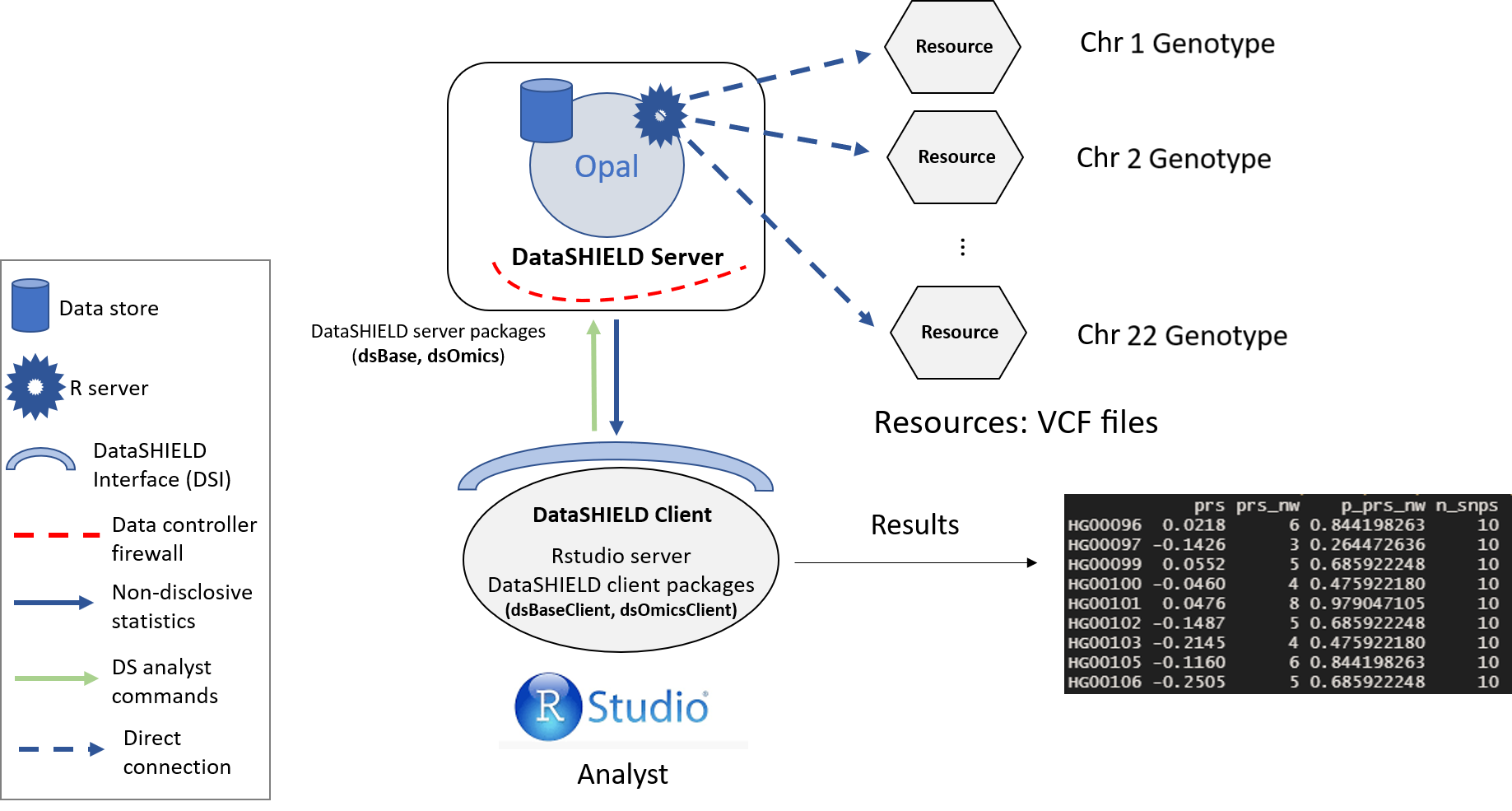
Figure 6.1: Proposed infrastructure to perform PRS studies.
6.3 Source of polygenic scores
There is a public repository of polygenic scores available at https://www.pgscatalog.org/, on this website there are 2155 different polygenic scores (January 2022) that have been extracted from curated literature. All those scores refer to 526 different traits. Due the relevance of this project, we made sure to include a way of sourcing it’s contents automatically.
There are two ways of stating the SNPs of interest and their weights in order to calculate the PRS.
Provide a PGS Catalog ‘Polygenic Score ID & Name’. If this option is in use, the SNPs and beta weights will be downloaded from the PGS Catalog and will be used to calculate the PRS. (Example:
PGS000008)Providing a
prs_table(SNPs of interest) table. Theprs_tabletable has to have a defined structure and column names in order to be understood by this function. This table can be formulated using two schemas:- Scheme 1: Provide SNP positions. Use the column names:
chr_name,chr_position,effect_allele,reference_allele,effect_weight.
chr_name chr_position effect_allele reference_allele effect_weight 1 100880328 T A 0.0373 1 121287994 G A -0.0673 6 152023191 A G 0.0626 … … … … … - Scheme 2: Provide SNP id’s. Use the column names:
rsID,effect_allele,reference_allele,effect_weight.
rdID effect_allele reference_allele effect_weight rs11206510 T C 0.0769 rs4773144 G A 0.0676 rs17514846 A C 0.0487 … … … … - Scheme 1: Provide SNP positions. Use the column names:
The effect_weight have to be the betas (log(OR)).
Please note when using a custom prs_table table that it is much faster to use the Schema 1, as the subset of the VCF files is miles faster to do using chromosome name and positions rather than SNP id’s.
6.4 Connection to the Opal server
We have to create an Opal connection object to the cohort server. We do that using the following functions.
require('DSI')
require('DSOpal')
require('dsBaseClient')
require('dsOmicsClient')

builder <- DSI::newDSLoginBuilder()
builder$append(server = "cohort1", url = "https://opal-demo.obiba.org/",
               user =  "dsuser", password = "P@ssw0rd",
               driver = "OpalDriver", profile = "omics")
builder$append(server = "cohort2", url = "https://opal-demo.obiba.org/",
               user =  "dsuser", password = "P@ssw0rd",
               driver = "OpalDriver", profile = "omics")
builder$append(server = "cohort3", url = "https://opal-demo.obiba.org/",
               user =  "dsuser", password = "P@ssw0rd",
               driver = "OpalDriver", profile = "omics")
logindata <- builder$build()
conns <- DSI::datashield.login(logins = logindata)
6.5 Assign the VCF resources
We assign the VCF and phenotypes resources.
# Cohort 1 resources
lapply(1:21, function(x){
  DSI::datashield.assign.resource(conns[1], paste0("chr", x), paste0("GWAS.chr", x,"A"))
  })
DSI::datashield.assign.resource(conns[1], "phenotypes_resource", "GWAS.ega_phenotypes_1")

# Cohort 2 resources
lapply(1:21, function(x){
  DSI::datashield.assign.resource(conns[2], paste0("chr", x), paste0("GWAS.chr", x,"B"))
  })
DSI::datashield.assign.resource(conns[2], "phenotypes_resource", "GWAS.ega_phenotypes_2")

# Cohort 3 resources
lapply(1:21, function(x){
  DSI::datashield.assign.resource(conns[3], paste0("chr", x), paste0("GWAS.chr", x,"C"))
  })
DSI::datashield.assign.resource(conns[3], "phenotypes_resource", "GWAS.ega_phenotypes_3")DSI::datashield.assign.expr(conns = conns, symbol = "phenotypes",
expr = as.symbol("as.resource.data.frame(phenotypes_resource)"))There is one crucial difference between this analysis and the GWAS, here we don’t need to resolve the resources. This is for memory efficiency purposes. When we calculate a PRS, we are only interested in a small selection of SNPs, for that reason the (potentially) huge VCF files will be trimmed before being resolved, so only the relevant SNPs are loaded in the memory. For that reason the resolving of the resources is delegated to the ds.PRS function, which will perform this trimming according to the SNPs of interest yielded by the PGS catalog query or the prs_table table. [CAMBIAR]
Finally the resources are resolved to retrieve the data in the remote sessions.
lapply(1:21, function(x){
  DSI::datashield.assign.expr(conns = conns, symbol = paste0("gds", x, "_object"),
                            expr = as.symbol(paste0("as.resource.object(chr", x, ")")))
})
6.6 Calculate the PRS
The PRS results will be added to the phenotypes table to be later studied using a pooled GLM. To do that, the following arguments of the function ds.PRS will be used:
table: Name of the table where the results will be merged.table_id_column: Number of the column in thetabletable that contains the individuals ID to merge the results from the PRS.table_prs_name: Name to append to the PRS results. It will take the structureprs_table_prs_nameandprs_nw_table_prs_name.
6.6.1 PGS Catalog Example
For this example we will calculate the PRS associated to the trait ‘HDL Cholesterol’ and ‘Thyroid cancer’, which corresponds to the PGS ID PGS000660 and PGS000636
resources <- paste0("gds", 1:21, "_object")

# HDL cholesterol
ds.PRS(resources = resources, pgs_id = "PGS000660",
       table = "phenotypes", table_id_column = "subject_id")
# Thyroid cancer
ds.PRS(resources = resources, pgs_id = "PGS000636",
       table = "phenotypes", table_id_column = "subject_id")
We can check that the results have been correctly added to the phenotypes table.
tail(ds.colnames('phenotypes')[[1]])[1] "prs_PGS000660" "prs_nw_PGS000660" "n_snps_PGS000660" "prs_PGS000636"
[5] "prs_nw_PGS000636" "n_snps_PGS000636"6.6.2 Custom prs_table example
Here we will illustrate a use case with a custom prs_table, please note that the proposed SNPs of interest and betas are totally arbitrary.
We will first assemble the prs_table table following the indications found on the Details section of ?ds.PRS (Schema 1).
prs_table <- data.frame(chr_name = c(9, 9, 9, 9, 1, 1, 2, 2),
                  chr_position = c(177034, 161674, 140859, 119681,
                                   60351, 825410, 154629, 145710),
                  effect_allele = c("T", "C", "G", "C", "G", "G", "T", "A"),
                  reference_allele = c("G", "T", "A", "T", "A", "A", "G", "G"),
                  effect_weight = c(0.5, 0.2, 0.1, 0.2, 0.1, 0.3, 0.1, 0.8))
Now we can pass the custom prs_table to the PRS function to retrieve the aggregated results.
resources <- paste0("gds", 1:21, "_object")

ds.PRS(resources = resources, prs_table = prs_table,
       table = "phenotypes", table_id_column = "subject_id",
       table_prs_name = "custom_prs_table_results")
6.7 Study of the PRS results
We can fit pooled GLM models using the function ds.glm. In this use case we will fit a model to relate the HDL.cholesterol to prs_PGS000660 adjusted by sex. The same will be done with the prs_PGS000636.
ds.glm(formula = "hdl_cholesterol ~ prs_PGS000660 + sex",
       family = "gaussian", data = "phenotypes")$coefficients
Estimate Std. Error z-value p-value low0.95CI
(Intercept) 1.576448314 0.178438076 8.8347081 1.003600e-18 1.22671611
prs_PGS000660 -0.003678982 0.009899804 -0.3716217 7.101746e-01 -0.02308224
sexmale 0.002311580 0.016140511 0.1432161 8.861195e-01 -0.02932324
high0.95CI
(Intercept) 1.92618052
prs_PGS000660 0.01572428
sexmale 0.03394640ds.glm(formula = "hdl_cholesterol ~ prs_PGS000636 + sex",
family = "gaussian", data = "phenotypes")$coefficients Estimate Std. Error z-value p-value low0.95CI
(Intercept) 1.522002437 0.01614425 94.2751901 0.0000000 1.49036028
prs_PGS000636 -0.066872228 0.06553929 -1.0203380 0.3075682 -0.19532688
sexmale 0.002416221 0.01613787 0.1497237 0.8809826 -0.02921342
high0.95CI
(Intercept) 1.55364459
prs_PGS000636 0.06158242
sexmale 0.03404586datashield.logout(conns)