10 Epigenome-wide association analysis (EWAS)
|
⚠️ RESOURCES USED ALONG THIS SECTION |
|||||||||
|---|---|---|---|---|---|---|---|---|---|
|
From https://opal-demo.obiba.org/ : |
|||||||||
|
In this section we will illustrate how to perform an epigenome-wide association analysis (EWAS) using methylation data. EWAS requires basically the same statistical methods as those used in DGE. It should be noticed that the pooled analysis we are going to illustrate here can also be performed with transcriptomic data, however the data needs to be harmonized beforehand to ensure each study has the same range values. For EWAS where methylation is measured using beta values (e.g CpG data are in the range 0-1) this is not a problem. In any case, adopting the meta-analysis approach could be a safe option without the need of harmonization.
Moreover, we encourage to perform pooled analysis only on the significant hits obtained by the meta-analysis, since it is a much slower methodology.
The data used in this section has been downloaded from GEO (accession number GSE66351) which contains DNA methylation profiling (Illumina 450K array) (section 3.4). Data corresponds to CpGs beta values measured in the superior temporal gyrus and prefrontal cortex brain regions of patients with Alzheimer’s.
This kind of data is encapsulated on a type of R object called ExpressionSet, this objects are part of the BioConductor project and are meant to contain different sources of genomic data, alongside the genomic data they can also contain the phenotypes and metadata associated to a study. Researchers who are not familiar with ExpressionSet can find further information here.
The data that we will be using along this section is an ExpressionSet objects. Notice that genomic data is encoded as beta-values that ensure data harmonization across studies.
In order to illustrate how to perform data analyses using federated data, we have split the data into two synthetic cohorts (split by individuals). We have created two resources on the demo Opal server called GSE66351_1 and GSE66351_2 respectively. They can be found inside the OMICS project. Some summaries of the datasets are the following:
| Cohort 1 | Cohort 2 | Total | |
|---|---|---|---|
| Number of CpGs | 481,868 | 481,868 | 481,868 |
| Number of individuals | 100 | 90 | 190 |
| Number of covariates | 49 | 49 | 49 |
| Number of annotation features | 37 | 37 | 37 |
The structure used is illustrated on the following figure.
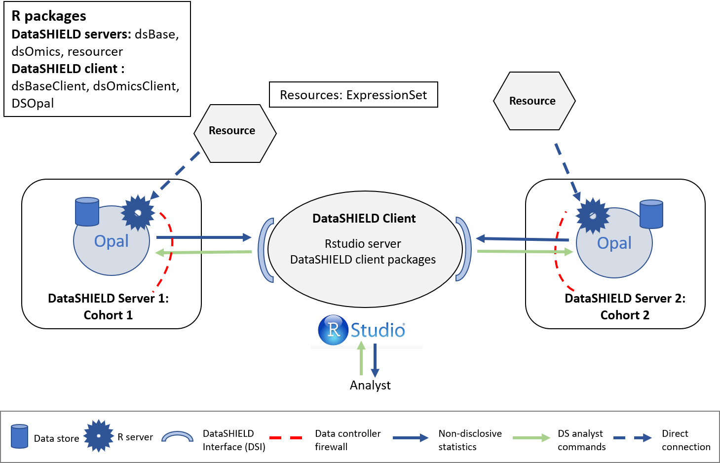
Figure 10.1: Proposed infrastructure to perform EWAS studies.
The data analyst corresponds to the “RStudio” session, which through DataSHIELD Interface (DSI) connects with the Opal server. The Opal servers contain a resource that correspond to the GEO:GSE66351 ExpressionSet (subseted by individuals).
We will illustrate the following use cases:
- Single CpG pooled analysis
- Multiple CpGs pooled analysis
- Full genome meta-analysis
- Full genome meta-analysis adjusting for surrogate variables
10.1 Initial steps for all use cases
10.1.1 Connection to the Opal server
We have to create an Opal connection object to the different cohorts server. We do that using the following functions.
require('DSI')
require('DSOpal')
require('dsBaseClient')
require('dsOmicsClient')

builder <- DSI::newDSLoginBuilder()
builder$append(server = "cohort1", url = "https://opal-demo.obiba.org/",
               user =  "dsuser", password = "P@ssw0rd",
               driver = "OpalDriver", profile = "omics")
builder$append(server = "cohort2", url = "https://opal-demo.obiba.org/",
               user =  "dsuser", password = "P@ssw0rd",
               driver = "OpalDriver", profile = "omics")
logindata <- builder$build()
conns <- DSI::datashield.login(logins = logindata)
It is important to note that in this use case, we are only using one server (https://opal-demo.obiba.org/), on this server there are all the resources that correspond to the different cohorts. On a more real scenario each one of the builder$append instructions would be connecting to a different server.
10.1.2 Assign the ExpressionSet resource
Now that we have created a connection object to the different Opals, we have started two R sessions, our analysis will take place on those remote sessions, so we have to load the data into them.
In this use case we will use 2 different resources from the OMICS project hosted on the demo Opal server. The names of the resources are GSE66351_X (where X is the cohort identifier 1/2). Following the Opal syntax, we will refer to them using the string OMICS.GSE66351_X.
We have to refer specifically to each different server by using conns[X], this allows us to communicate with the server of interest to indicate to it the resource that it has to load.
# Cohort 1 resource load
DSI::datashield.assign.resource(conns[1], "eSet_resource", "OMICS.GSE66351_1")

# Cohort 2 resource load
DSI::datashield.assign.resource(conns[2], "eSet_resource", "OMICS.GSE66351_2")
Now we have assigned all the resources named into our remote R sessions. We have assigned them to the variables called eSet_resource. To verify this step has been performed correctly, we can use the ds.class function to check for their class and that they exist on the remote sessions.
ds.class("eSet_resource")$cohort1
[1] "RDataFileResourceClient" "FileResourceClient"
[3] "ResourceClient" "R6"
$cohort2
[1] "RDataFileResourceClient" "FileResourceClient"
[3] "ResourceClient" "R6" We can see that the object eSet_resource exists in both servers.
Finally the resource is resolved to retrieve the data in the remote sessions.
DSI::datashield.assign.expr(conns = conns, symbol = "eSet",
                            expr = as.symbol("as.resource.object(eSet_resource)"))
Now we have resolved the resource named eSet_resource into our remote R session. The object retrieved has been assigned into the variable named eSet. We can check the process was successful as we did before.
ds.class("eSet")$cohort1
[1] "ExpressionSet"
attr(,"package")
[1] "Biobase"
$cohort2
[1] "ExpressionSet"
attr(,"package")
[1] "Biobase"10.1.3 Inspect the ExpressionSet
Feature names can be returned by:
fn <- ds.featureNames("eSet")
lapply(fn, head)
$cohort1
[1] "cg00000029" "cg00000108" "cg00000109" "cg00000165" "cg00000236"
[6] "cg00000289"
$cohort2
[1] "cg00000029" "cg00000108" "cg00000109" "cg00000165" "cg00000236"
[6] "cg00000289"Experimental phenotypes variables can be obtained by:
fn <- ds.varLabels("eSet")
lapply(fn, head)
$cohort1
[1] "title" "geo_accession" "status" "submission_date"
[5] "last_update_date" "type"
$cohort2
[1] "title" "geo_accession" "status" "submission_date"
[5] "last_update_date" "type" The columns of the annotation can be obtained by:
fn <- ds.fvarLabels("eSet")
lapply(fn, head)
$cohort1
[1] "ID" "Name" "AddressA_ID" "AlleleA_ProbeSeq"
[5] "AddressB_ID" "AlleleB_ProbeSeq"
$cohort2
[1] "ID" "Name" "AddressA_ID" "AlleleA_ProbeSeq"
[5] "AddressB_ID" "AlleleB_ProbeSeq"10.2 Single CpG pooled analysis
Once the methylation data have been loaded into the opal server, we can perform different type of analyses using functions from the dsOmicsClient package. Let us start by illustrating how to analyze a single CpG from two cohorts by using an approach that is mathematically equivalent to placing all individual-level (pooled).
ans <- ds.lmFeature(feature = "cg07363416",
                    model = ~ diagnosis + Sex,
                    Set = "eSet",
                    datasources = conns)
ans
Estimate Std. Error p-value
cg07363416 0.03459886 0.02504291 0.1670998
attr(,"class")
[1] "dsLmFeature" "matrix" "array" 10.3 Multiple CpGs pooled analysis
The same analysis can be performed for multiple features. This process can be parallelized using mclapply function from the multicore package (only works on GNU/Linux, not on Windows).
ans <- ds.lmFeature(feature = c("cg00000029", "cg00000108", "cg00000109", "cg00000165"),
                    model = ~ diagnosis + Sex,
                    Set = "eSet",
                    datasources = conns,
                    mc.cores = 20)
If the feature argument is not supplied, all the features will be analyzed, please note that this process can be extremely slow if there is a huge number of features; for example, on the case we are illustrating we have over 400K features, so this process would take too much time.
If all the features are to be studied, we recommend switching to meta-analysis methods. More information on the next section.
10.4 Full genome meta-analysis
We can adopt another strategy that is to run a glm of each feature independently at each study using limma package (which is really fast) and then combine the results (i.e. meta-analysis approach).
ans.limma <- ds.limma(model = ~ diagnosis + Sex,
                      Set = "eSet",
                      datasources = conns)
Then, we can visualize the top genes at each study (i.e server) by:
lapply(ans.limma, head)$cohort1
# A tibble: 6 x 7
id n beta SE t P.Value adj.P.Val
<chr> <int> <dbl> <dbl> <dbl> <dbl> <dbl>
1 cg13138089 100 -0.147 0.0122 -6.62 0.00000000190 0.000466
2 cg23859635 100 -0.0569 0.00520 -6.58 0.00000000232 0.000466
3 cg13772815 100 -0.0820 0.0135 -6.50 0.00000000327 0.000466
4 cg12706938 100 -0.0519 0.00872 -6.45 0.00000000425 0.000466
5 cg24724506 100 -0.0452 0.00775 -6.39 0.00000000547 0.000466
6 cg02812891 100 -0.125 0.0163 -6.33 0.00000000731 0.000466
$cohort2
# A tibble: 6 x 7
id n beta SE t P.Value adj.P.Val
<chr> <int> <dbl> <dbl> <dbl> <dbl> <dbl>
1 cg04046629 90 -0.101 0.0128 -5.91 0.0000000621 0.0172
2 cg07664323 90 -0.0431 0.00390 -5.85 0.0000000822 0.0172
3 cg27098804 90 -0.0688 0.0147 -5.79 0.000000107 0.0172
4 cg08933615 90 -0.0461 0.00791 -5.55 0.000000298 0.0360
5 cg18349298 90 -0.0491 0.00848 -5.42 0.000000507 0.0489
6 cg02182795 90 -0.0199 0.0155 -5.36 0.000000670 0.0538The annotation can be added by using the argument annotCols. It should be a vector with the columns of the annotation available in the ExpressionSet or RangedSummarizedExperiment that want to be showed. To obtain the available annotation columns revisit #ewas-inspect.
ans.limma.annot <- ds.limma(model = ~ diagnosis + Sex,
                            Set = "eSet",
                            annotCols = c("CHR", "UCSC_RefGene_Name"),
                            datasources = conns)
lapply(ans.limma.annot, head)
$cohort1
# A tibble: 6 x 9
id n beta SE t P.Value adj.P.Val CHR UCSC_RefGene_Na~
<chr> <int> <dbl> <dbl> <dbl> <dbl> <dbl> <chr> <chr>
1 cg1313~ 100 -0.147 0.0122 -6.62 1.90e-9 0.000466 2 "ECEL1P2"
2 cg2385~ 100 -0.0569 0.00520 -6.58 2.32e-9 0.000466 2 "MTA3"
3 cg1377~ 100 -0.0820 0.0135 -6.50 3.27e-9 0.000466 17 ""
4 cg1270~ 100 -0.0519 0.00872 -6.45 4.25e-9 0.000466 19 "MEX3D"
5 cg2472~ 100 -0.0452 0.00775 -6.39 5.47e-9 0.000466 19 "ISOC2;ISOC2;IS~
6 cg0281~ 100 -0.125 0.0163 -6.33 7.31e-9 0.000466 2 "ECEL1P2"
$cohort2
# A tibble: 6 x 9
id n beta SE t P.Value adj.P.Val CHR UCSC_RefGene_Na~
<chr> <int> <dbl> <dbl> <dbl> <dbl> <dbl> <chr> <chr>
1 cg0404~ 90 -0.101 0.0128 -5.91 6.21e-8 0.0172 11 "CD6"
2 cg0766~ 90 -0.0431 0.00390 -5.85 8.22e-8 0.0172 6 "MUC21"
3 cg2709~ 90 -0.0688 0.0147 -5.79 1.07e-7 0.0172 11 "CD6"
4 cg0893~ 90 -0.0461 0.00791 -5.55 2.98e-7 0.0360 1 ""
5 cg1834~ 90 -0.0491 0.00848 -5.42 5.07e-7 0.0489 3 "RARRES1;RARRES~
6 cg0218~ 90 -0.0199 0.0155 -5.36 6.70e-7 0.0538 8 "" Then, the last step is to meta-analyze the results. Different methods can be used to this end. We have implemented a method that meta-analyze the p-pvalues of each study as follows:
ans.meta <- metaPvalues(ans.limma)
ans.meta
# A tibble: 481,868 x 4
id cohort1 cohort2 p.meta
<chr> <dbl> <dbl> <dbl>
1 cg13138089 0.00000000190 0.00000763 4.78e-13
2 cg25317941 0.0000000179 0.00000196 1.12e-12
3 cg02812891 0.00000000731 0.00000707 1.63e-12
4 cg12706938 0.00000000425 0.0000161 2.14e-12
5 cg16026647 0.000000101 0.000000797 2.51e-12
6 cg12695465 0.00000000985 0.0000144 4.33e-12
7 cg21171625 0.000000146 0.00000225 9.78e-12
8 cg13772815 0.00000000327 0.000122 1.18e-11
9 cg00228891 0.000000166 0.00000283 1.38e-11
10 cg21488617 0.0000000186 0.0000299 1.62e-11
# ... with 481,858 more rowsWe can verify that the results are pretty similar to those obtained using pooled analyses. Here we compute the association for the top two CpGs:
res <- ds.lmFeature(feature = ans.meta$id[1:2],
                     model = ~ diagnosis + Sex,
                     Set = "eSet",
                     datasources = conns)
res
Estimate Std. Error p-value p.adj
cg25317941 -0.03452376 0.004303781 1.042679e-15 1.057482e-15
cg13138089 -0.13733479 0.017124046 1.057482e-15 1.057482e-15
attr(,"class")
[1] "dsLmFeature" "matrix" "array" We can create a QQ-plot by using the function qqplot available in our package.
qqplot(ans.meta$p.meta)
Here In some cases inflation can be observed, so that, correction for cell-type or surrogate variables must be performed. We describe how we can do that in the next two sections.
10.5 Adjusting for surrogate variables
The vast majority of omic studies require to control for unwanted variability. The surrogate variable analysis (SVA) can address this issue by estimating some hidden covariates that capture differences across individuals due to some artifacts such as batch effects or sample quality among others. The method is implemented in SVA package.
Performing this type of analysis using the ds.lmFeature function is not allowed since estimating SVA would require to implement a non-disclosive method that computes SVA from the different servers. This will be a future topic of the dsOmicsClient. For that reason we have to adopt a compromise solution which is to perform the SVA independently at each study. We use the ds.limma function to perform the analyses adjusted for SVA at each study.
ans.sva <- ds.limma(model = ~ diagnosis + Sex,
                    Set = "eSet",
                    sva = TRUE, annotCols = c("CHR", "UCSC_RefGene_Name"))
ans.sva
$cohort1
# A tibble: 481,868 x 9
id n beta SE t P.Value adj.P.Val CHR UCSC_RefGene_Na~
<chr> <int> <dbl> <dbl> <dbl> <dbl> <dbl> <chr> <chr>
1 cg1313~ 100 -0.147 0.0122 -6.62 1.90e-9 0.000466 2 "ECEL1P2"
2 cg2385~ 100 -0.0569 0.00520 -6.58 2.32e-9 0.000466 2 "MTA3"
3 cg1377~ 100 -0.0820 0.0135 -6.50 3.27e-9 0.000466 17 ""
4 cg1270~ 100 -0.0519 0.00872 -6.45 4.25e-9 0.000466 19 "MEX3D"
5 cg2472~ 100 -0.0452 0.00775 -6.39 5.47e-9 0.000466 19 "ISOC2;ISOC2;IS~
6 cg0281~ 100 -0.125 0.0163 -6.33 7.31e-9 0.000466 2 "ECEL1P2"
7 cg2766~ 100 -0.0588 0.0198 -6.33 7.48e-9 0.000466 16 "ANKRD11"
8 cg1537~ 100 -0.0709 0.0115 -6.32 7.83e-9 0.000466 2 "LPIN1"
9 cg1552~ 100 -0.0446 0.00750 -6.29 8.69e-9 0.000466 10 ""
10 cg1269~ 100 -0.0497 0.00155 -6.27 9.85e-9 0.000475 6 "GCNT2;GCNT2;GC~
# ... with 481,858 more rows
$cohort2
# A tibble: 481,868 x 9
id n beta SE t P.Value adj.P.Val CHR UCSC_RefGene_Name
<chr> <int> <dbl> <dbl> <dbl> <dbl> <dbl> <chr> <chr>
1 cg040~ 90 -0.101 0.0128 -5.91 6.21e-8 0.0172 11 "CD6"
2 cg076~ 90 -0.0431 0.00390 -5.85 8.22e-8 0.0172 6 "MUC21"
3 cg270~ 90 -0.0688 0.0147 -5.79 1.07e-7 0.0172 11 "CD6"
4 cg089~ 90 -0.0461 0.00791 -5.55 2.98e-7 0.0360 1 ""
5 cg183~ 90 -0.0491 0.00848 -5.42 5.07e-7 0.0489 3 "RARRES1;RARRES1"
6 cg021~ 90 -0.0199 0.0155 -5.36 6.70e-7 0.0538 8 ""
7 cg160~ 90 -0.0531 0.0196 -5.31 7.97e-7 0.0548 17 "MEIS3P1"
8 cg012~ 90 -0.0537 0.00971 -5.18 1.39e-6 0.0582 7 "HOXA2"
9 cg251~ 90 -0.0224 0.00736 -5.15 1.57e-6 0.0582 3 "ZBTB20;ZBTB20;ZB~
10 cg074~ 90 -0.0475 0.00166 -5.13 1.67e-6 0.0582 22 "C22orf27"
# ... with 481,858 more rows
attr(,"class")
[1] "dsLimma" "list" Then, data can be combined meta-anlyzed as follows:
ans.meta.sv <- metaPvalues(ans.sva)
ans.meta.sv
# A tibble: 481,868 x 4
id cohort1 cohort2 p.meta
<chr> <dbl> <dbl> <dbl>
1 cg13138089 0.00000000190 0.00000763 4.78e-13
2 cg25317941 0.0000000179 0.00000196 1.12e-12
3 cg02812891 0.00000000731 0.00000707 1.63e-12
4 cg12706938 0.00000000425 0.0000161 2.14e-12
5 cg16026647 0.000000101 0.000000797 2.51e-12
6 cg12695465 0.00000000985 0.0000144 4.33e-12
7 cg21171625 0.000000146 0.00000225 9.78e-12
8 cg13772815 0.00000000327 0.000122 1.18e-11
9 cg00228891 0.000000166 0.00000283 1.38e-11
10 cg21488617 0.0000000186 0.0000299 1.62e-11
# ... with 481,858 more rowsAnd we can revisit the qqplot:
qqplot(ans.meta.sv$p.meta)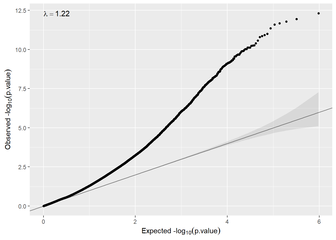
The DataSHIELD session must be closed by:
datashield.logout(conns)