9 Differential gene expression (DGE) analysis
|
⚠️ RESOURCES USED ALONG THIS SECTION |
||||||
|---|---|---|---|---|---|---|
|
From https://opal-demo.obiba.org/ : |
||||||
|
In this section we will illustrate how to perform transcriptomic data analysis using data from TCGA project (section 3.3). We have uploaded to the demo Opal server a resource called tcga_liver whose URL is http://duffel.rail.bio/recount/TCGA/rse_gene_liver.Rdata which is available through the recount project. The resource used on this section contains a RangedSummarizedExperimentwith the RNAseq profiling of liver cancer data from TCGA.
The resource is located inside the OMICS project. Some summaries of the dataset are the following:
| TCGA Liver data | |
|---|---|
| Number of individuals | 424 |
| Number of genes | 58,037 |
| Number of covariate fields | 864 |
The structure used is illustrated on the following figure.
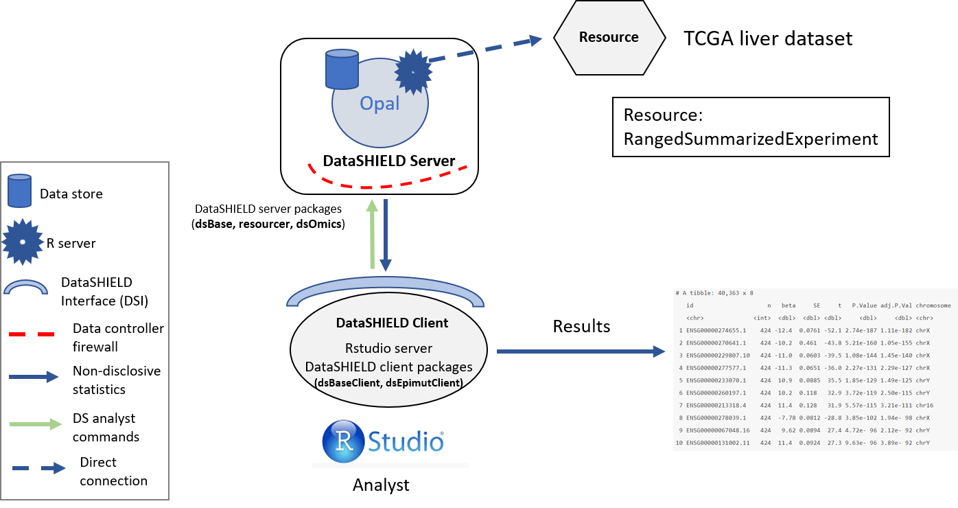
Figure 9.1: Proposed infrastructure to perform DGE studies.
We illustrate a differential expression analysis to compare RNAseq profiling of women vs men (variable gdc_cases.demographic.gender). The DGE analysis is normally performed using limma package. In that case, as we are analyzing RNA-seq data, limma + voom method will be required.
The following use cases will be illustrated:
- DGE analysis
- DGE analysis adjusting for surrogate variables
9.1 Connection to the Opal server
We have to create an Opal connection object to the cohort server. We do that using the following functions.
require('DSI')
require('DSOpal')
require('dsBaseClient')
require('dsOmicsClient')

builder <- DSI::newDSLoginBuilder()
builder$append(server = "cohort1", url = "https://opal-demo.obiba.org/",
               user =  "dsuser", password = "P@ssw0rd",
               driver = "OpalDriver", profile = "omics")
logindata <- builder$build()
conns <- DSI::datashield.login(logins = logindata)
9.2 Assign the RSE resource
Now that we have created a connection object to the Opal, we have started a new R session on the server, our analysis will take place in this remote session, so we have to load the data into it.
In this use case we will use one resource from the OMICS project hosted on the demo Opal server. This resources correspond to RangedsummarizedExperiment dataset. The names of the resource is tcga_liver, we will refer to it using the string OMICS.tcga_liver.
DSI::datashield.assign.resource(conns, "rse_resource", "OMICS.tcga_liver")Now we have assigned the resource named OMICS.tcga_liver into our remote R session. We have assigned it to a variable called rse_resource. To verify this step has been performed correctly, we could use the ds.class function to check for their class and that they exist on the remote sessions.
ds.class("rse_resource")$cohort1
[1] "RDataFileResourceClient" "FileResourceClient"
[3] "ResourceClient" "R6" We can see that the object rse_resource exists in the server.
Finally the resource is resolved to retrieve the data in the remote session.
DSI::datashield.assign.expr(conns = conns, symbol = "rse",
                            expr = as.symbol("as.resource.object(rse_resource)"))
Now we have resolved the resource named rse_resource into our remote R session. The object retrieved has been assigned into the variable named rse. We can check the process was successful as we did before.
ds.class("rse")$cohort1
[1] "RangedSummarizedExperiment"
attr(,"package")
[1] "SummarizedExperiment"9.3 Inspect the RSE
The number of features and samples can be inspected with:
ds.dim("rse")$`dimensions of rse in cohort1`
[1] 58037 424
$`dimensions of rse in combined studies`
[1] 58037 424And the names of the features using the same function used in the case of analyzing an ExpressionSet:
name.features <- ds.featureNames("rse")
lapply(name.features, head)
$cohort1
[1] "ENSG00000000003.14" "ENSG00000000005.5" "ENSG00000000419.12"
[4] "ENSG00000000457.13" "ENSG00000000460.16" "ENSG00000000938.12"Also the covariate names can be inspected by:
name.vars <- ds.featureData("rse")
lapply(name.vars, head, n=15)
$cohort1
[1] "project"
[2] "sample"
[3] "experiment"
[4] "run"
[5] "read_count_as_reported_by_sra"
[6] "reads_downloaded"
[7] "proportion_of_reads_reported_by_sra_downloaded"
[8] "paired_end"
[9] "sra_misreported_paired_end"
[10] "mapped_read_count"
[11] "auc"
[12] "sharq_beta_tissue"
[13] "sharq_beta_cell_type"
[14] "biosample_submission_date"
[15] "biosample_publication_date" We can visualize the levels of the variable having gender information that will be our condition (i.e., we are interested in obtaining genes that are differentially expressed between males and females).
ds.table1D("rse$gdc_cases.demographic.gender")$counts
rse$gdc_cases.demographic.gender
female 143
male 281
Total 424
$percentages
rse$gdc_cases.demographic.gender
female 33.73
male 66.27
Total 100.00
$validity
[1] "All tables are valid!"9.4 Pre-processing for RNAseq data
We have implemented a function called ds.RNAseqPreproc() to perform RNAseq data pre-processing that includes:
- Transforming data into log2 CPM units
- Filtering lowly-expressed genes
- Data normalization
ds.RNAseqPreproc('rse', group = 'gdc_cases.demographic.gender',
                 newobj.name = 'rse.pre')
Note that it is recommended to indicate the grouping variable (i.e., condition). Once data has been pre-processed, we can perform differential expression analysis. Notice how dimensions have changed given the fact that we have removed genes with low expression which are expected to do not be differentially expressed.
ds.dim('rse')$`dimensions of rse in cohort1`
[1] 58037 424
$`dimensions of rse in combined studies`
[1] 58037 424ds.dim('rse.pre')$`dimensions of rse.pre in cohort1`
[1] 40363 424
$`dimensions of rse.pre in combined studies`
[1] 40363 4249.5 DGE analysis
The differential expression analysis in dsOmicsClient/dsOmics is implemented in the funcion ds.limma(). This functions runs a limma-pipeline for microarray data and for RNAseq data allows:
- oom + limma
- DESeq2
- edgeR
We recommend to use the voom + limma pipeline proposed here given its versatility and that limma is much faster than DESeq2 and edgeR. By default, the function considers that data is obtained from a microarray experiment (type.data = "microarray"). Therefore, as we are analyzing RNAseq data, we must indicate that type.data = "RNAse".
ans.gender <- ds.limma(model =  ~ gdc_cases.demographic.gender,
                       Set = "rse.pre", type.data = "RNAseq")
The top differentially expressed genes can be visualized by:
ans.gender$cohort1
# A tibble: 40,363 x 7
id n beta SE t P.Value adj.P.Val
<chr> <int> <dbl> <dbl> <dbl> <dbl> <dbl>
1 ENSG00000274655.1 424 -12.4 0.0761 -52.1 2.74e-187 1.11e-182
2 ENSG00000270641.1 424 -10.2 0.461 -43.8 5.21e-160 1.05e-155
3 ENSG00000229807.10 424 -11.0 0.0603 -39.5 1.08e-144 1.45e-140
4 ENSG00000277577.1 424 -11.3 0.0651 -36.0 2.27e-131 2.29e-127
5 ENSG00000233070.1 424 10.9 0.0885 35.5 1.85e-129 1.49e-125
6 ENSG00000260197.1 424 10.2 0.118 32.9 3.72e-119 2.50e-115
7 ENSG00000213318.4 424 11.4 0.128 31.9 5.57e-115 3.21e-111
8 ENSG00000278039.1 424 -7.78 0.0812 -28.8 3.85e-102 1.94e- 98
9 ENSG00000067048.16 424 9.62 0.0894 27.4 4.72e- 96 2.12e- 92
10 ENSG00000131002.11 424 11.4 0.0924 27.3 9.63e- 96 3.89e- 92
# ... with 40,353 more rows
attr(,"class")
[1] "dsLimma" "list" We can verify whether the distribution of the observed p-values are the ones we expect in this type of analyses:
hist(ans.gender$cohort1$P.Value, xlab="Raw p-value gender effect",
     main="", las=1, cex.lab=1.5, cex.axis=1.2, col="gray")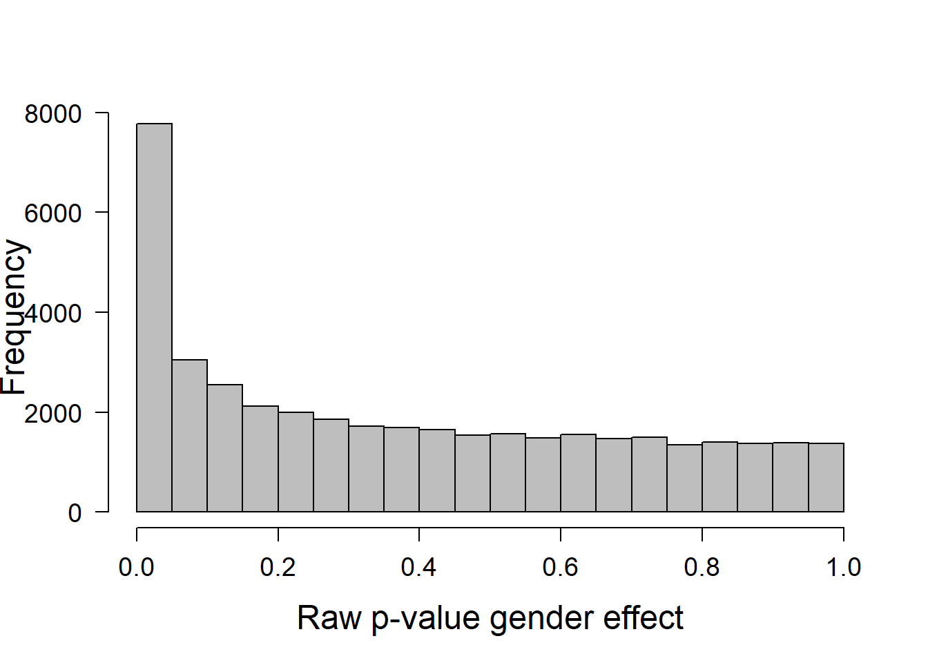
9.6 Surrogate variable analysis
We can also check whether there is inflation just executing
qqplot(ans.gender$cohort1$P.Value)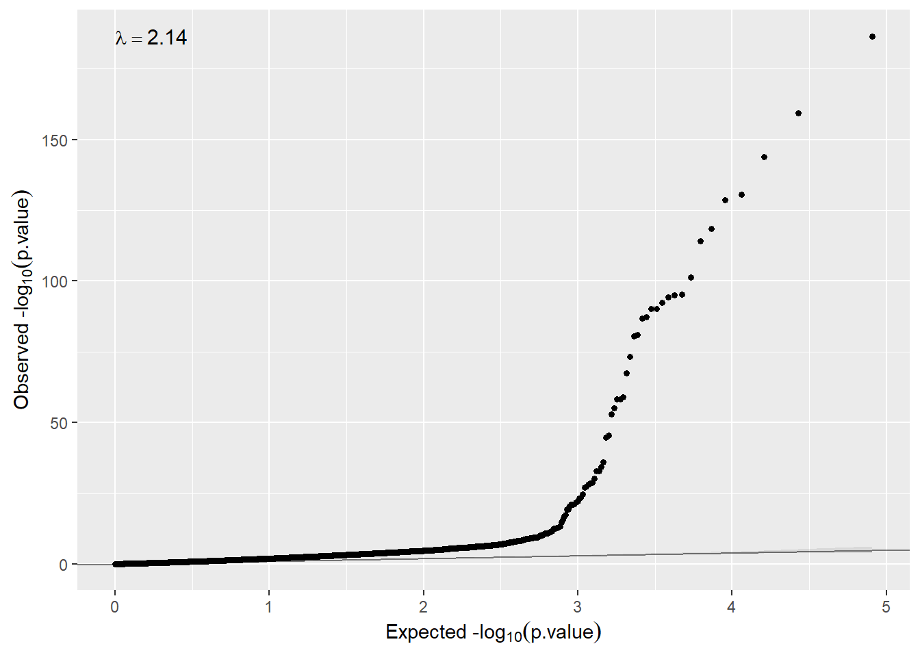
So, in that case, the model needs to remove unwanted variability (\(\lambda > 2\)). If so, we can use surrogate variable analysis just changing the argument sva=TRUE.
ans.gender.sva <- ds.limma(model =  ~ gdc_cases.demographic.gender,
                       Set = "rse.pre", type.data = "RNAseq",
                       sva = TRUE)
Now the inflation has dramatically been reduced (\(\lambda > 1.12\)).
qqplot(ans.gender.sva$cohort1$P.Value)
We can add annotation to the output that is available in our RSE object. We can have access to this information by:
ds.fvarLabels('rse.pre')$cohort1
[1] "chromosome" "start" "end" "width" "strand"
[6] "gene_id" "bp_length" "symbol"
attr(,"class")
[1] "dsfvarLabels" "list" So, we can run:
ans.gender.sva <- ds.limma(model =  ~ gdc_cases.demographic.gender,
                       Set = "rse.pre", type.data = "RNAseq",
                       sva = TRUE, annotCols = c("chromosome"))
The results are:
ans.gender.sva$cohort1
# A tibble: 40,363 x 8
id n beta SE t P.Value adj.P.Val chromosome
<chr> <int> <dbl> <dbl> <dbl> <dbl> <dbl> <chr>
1 ENSG00000274655.1 424 -12.4 0.0761 -52.1 2.74e-187 1.11e-182 chrX
2 ENSG00000270641.1 424 -10.2 0.461 -43.8 5.21e-160 1.05e-155 chrX
3 ENSG00000229807.10 424 -11.0 0.0603 -39.5 1.08e-144 1.45e-140 chrX
4 ENSG00000277577.1 424 -11.3 0.0651 -36.0 2.27e-131 2.29e-127 chrX
5 ENSG00000233070.1 424 10.9 0.0885 35.5 1.85e-129 1.49e-125 chrY
6 ENSG00000260197.1 424 10.2 0.118 32.9 3.72e-119 2.50e-115 chrY
7 ENSG00000213318.4 424 11.4 0.128 31.9 5.57e-115 3.21e-111 chr16
8 ENSG00000278039.1 424 -7.78 0.0812 -28.8 3.85e-102 1.94e- 98 chrX
9 ENSG00000067048.16 424 9.62 0.0894 27.4 4.72e- 96 2.12e- 92 chrY
10 ENSG00000131002.11 424 11.4 0.0924 27.3 9.63e- 96 3.89e- 92 chrY
# ... with 40,353 more rows
attr(,"class")
[1] "dsLimma" "list" The function has another arguments that can be used to fit other type of models:
sva: estimate surrogate variablesannotCols: to add annotation available in themethod: Linear regression (“ls”) or robust regression (“robust”) used in limma (lmFit)robust: robust method used for outlier sample variances used inlimma(eBayes)normalization: normalization method used in thevoomtransformation (default“none”)voomQualityWeights: shouldvoomQualityWeightsfunction be used instead ofvoom? (defaultFALSE)big: shouldSmartSVAbe used instead ofSVA(useful for big sample size or when analyzing epigenome data. DefaultFALSE)
We have also implemented two other functions ds.DESeq2 and ds.edgeR that perform DGE analysis using DESeq2 and edgeR methods. This is the R code used to that purpose:
To be supplied
We close the DataSHIELD session by:
datashield.logout(conns)