5 Genome wide association study (GWAS) analysis
Three different use cases will be illustrated in this section:
- Single cohort GWAS. Using data from all the individuals.
- Multi-cohort GWAS. Using the same individuals as the single cohort separated into three synthetic cohorts.
- Polygenic risk score. Using data from all the individuals.
For this, we will be using data from the CINECA project presented in the section 3.1. For all the illustrated cases we will use data divided by chromosome (VCF files). The procedure is the same if all the variants are on a single VCF. The phenotype information used throughout this section is not contained inside the VCF files mentioned previously, it is contained using traditional CSV/Excel files. This is to replicate the typical scenario where an investigator receives the genomic and phenotype data separated and has to merge it to study a specific relationship between the gene expression / variants and a certain phenotype.
5.1 Single cohort
|
⚠️ RESOURCES USED ALONG THIS SECTION |
|||||||||
|---|---|---|---|---|---|---|---|---|---|
|
From https://opal-demo.obiba.org/ : |
|||||||||
|
The single cohort analysis is a way of performing a GWAS study guaranteeing GDPR data confidentiality. The structure followed is illustrated on the following figure.
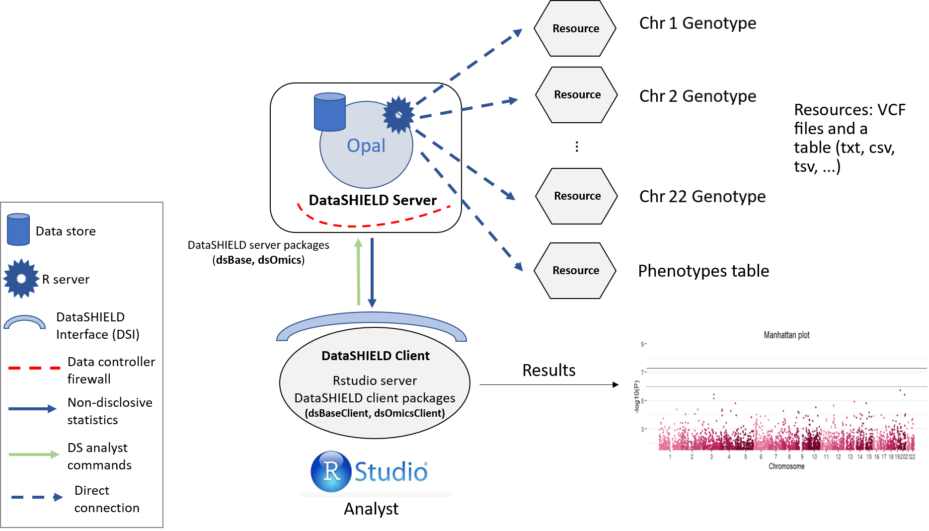
Figure 5.1: Proposed infrastructure to perform single-cohort GWAS studies.
The data analyst corresponds to the “RStudio” session, which through DataSHIELD Interface (DSI) connects with the Opal server located at the cohort network. This Opal server contains an array of resources that correspond to the different VCF files (sliced by chromosome) 1 and a resource that corresponds to the phenotypes table of the studied individuals.
5.1.1 Connection to the Opal server
We have to create an Opal connection object to the cohort server. We do that using the following functions.
require('DSI')
require('DSOpal')
require('dsBaseClient')
require('dsOmicsClient')

builder <- DSI::newDSLoginBuilder()
builder$append(server = "cohort1", url = "https://opal-demo.obiba.org/",
               user =  "dsuser", password = "P@ssw0rd",
               driver = "OpalDriver", profile = "omics")
logindata <- builder$build()
conns <- DSI::datashield.login(logins = logindata)
5.1.2 Assign the VCF resources
Now that we have created a connection object to the Opal, we have started a new R session on the server, our analysis will take place in this remote session, so we have to load the data into it.
In this use case we will use 21 different resources from the GWAS project hosted on the demo Opal server. This resources correspond to VCF files with information on individual chromosomes. The names of the resources are chrXX (where XX is the chromosome number). Following the Opal syntax, we will refer to them using the string GWAS.chrXX.
To load the resources we will use the DSI::datashield.assign.resource() function. Note that along the use case we use the lapply function to simplify our code since we have to perform repetitive operations. lapply is a way of creating loops in R, for more information visit the documentation.
lapply(1:21, function(x){
  DSI::datashield.assign.resource(conns, paste0("chr", x), paste0("GWAS.chr", x))
  })
Now we have assigned all the resources named GWAS.chrXX into our remote R session. We have assigned them to the variables called chrXX. To verify this step has been performed correctly, we could use the ds.class function to check for their class and that they exist on the remote session.
ds.class("chr1")$cohort1
[1] "GDSFileResourceClient" "FileResourceClient" "ResourceClient"
[4] "R6" To resolve the resources and retrieve the data in the remote session we will use the DSI::datashield.assign.expr() function. This function runs a line of code on the remote session 2, and in particular we want to run the function as.resource.object(), which is the DataSHIELD function in charge of resolving the resources.
lapply(1:21, function(x){
  DSI::datashield.assign.expr(conns = conns, symbol = paste0("gds", x, "_object"),
                            expr = as.symbol(paste0("as.resource.object(chr", x, ")")))
})
Now we have resolved the resources named chrXX into our remote R session. The objects retrieved have been assigned into variables named gdsXX_object. We can check the process was successful as we did before.
ds.class("gds1_object")$cohort1
[1] "GdsGenotypeReader"
attr(,"package")
[1] "GWASTools"5.1.3 Assign the phenotypes
The objects we have loaded into our remote session are VCF files that contain genomic information of the individuals. To perform a GWAS this information has to be related to some phenotypes to extract relationships. Therefore, we need to load the phenotypes into the remote session. The phenotypes information is a table that contains the individuals as rows and phenotypes as columns. In this use case, we will use a resource (as with the VCF files) to load the phenotypes table into the remote session.
The procedure is practically the same as before with some minor tweaks. To begin, we have the phenotypes information in a single table (hence, a single resource). Then, instead of using the function as.resource.object, we will use as.resource.data.frame, this is because before we were loading a special object (VCF file) and now we are loading a plain table, so the internal treatment on the remote session has to be different.
DSI::datashield.assign.resource(conns, "pheno", "GWAS.ega_phenotypes")
DSI::datashield.assign.expr(conns = conns, symbol = "pheno_object",
                            expr = quote(as.resource.data.frame(pheno)))
We can follow the same analogy as before to know that we have assigned the phenotypes table to a variable called pheno_object on the remote R session.
ds.class("pheno_object")$cohort1
[1] "spec_tbl_df" "tbl_df" "tbl" "data.frame" We can also check the column names to see which information is present on the table.
ds.colnames("pheno_object")[[1]] [1] "age_cancer_diagnosis" "age_recruitment"
[3] "alcohol_day" "basophill_count"
[5] "behaviour_tumour" "bmi"
[7] "c_reactive_protein_reportability" "record_origin"
[9] "report_format" "cholesterol"
[11] "birth_country" "actual_tobacco_smoker"
[13] "date_diagnosis" "diabetes_diagnosed_doctor"
[15] "diastolic_blood_pressure" "duration_moderate_activity"
[17] "duration_vigorous_activity" "energy"
[19] "eosinophill_count" "ethnicity"
[21] "ever_smoked" "fasting_time"
[23] "alcohol_frequency" "hdl_cholesterol"
[25] "hip_circumference" "histology_tumour"
[27] "home_e_coordinate" "home_n_coordinate"
[29] "e_house_score" "s_house_score"
[31] "w_house_score" "e_income_score"
[33] "w_income_score" "ldl_direct"
[35] "lymphocyte_count" "monocyte_count"
[37] "neutrophill_count" "n_accidental_death_close_gen_family"
[39] "household_count" "children_count"
[41] "operations_count" "operative_procedures"
[43] "past_tobacco" "platelet_count"
[45] "pulse_rate" "qualification"
[47] "cancer_occurrences" "reticulocuyte_count"
[49] "sleep_duration" "height"
[51] "subject_id" "triglycerides"
[53] "cancer_type_idc10" "cancer_type_idc9"
[55] "weight" "leukocyte_count"
[57] "sex" "phenotype"
[59] "age_death" "age_diagnosis_diabetes"
[61] "date_k85_report" "date_k86_report"
[63] "date_death" "enm_diseases"
[65] "source_k85_report" "source_k86_report"
[67] "age_hbp_diagnosis" "mental_disorders"
[69] "respiratory_disorders" "cancer_year"
[71] "circulatory_disorders" "digestive_disorders"
[73] "nervous_disorders" "immune_disorders" 5.1.4 Merge VCF (genotype) and phenotype information
Arrived at this point, we have 21 VCF objects (each one corresponds to a chromosome) and a phenotypes table on our remote session. The next step is merging each of the VCF objects with the phenotypes table. Before doing that however, we have to gather some information from the phenotypes table. The information to gather is summarized on the Table 5.1.
| Information | Details |
|---|---|
| Which column has the samples identifier? | Column name that contains the IDs of the samples. Those are the IDs that will be matched to the ones present on the VCF objects. |
| Which is the sex column on the covariates file? | Column name that contains the sex information. |
| How are males and how are females encoded into this column? | There is not a standard way to encode the sex information, some people use 0/1; male/female; etc. Our approach uses a library that requires a specific encoding, for that reason we need to know the original encoding to perform the translation. |
| Which is the case-control column? | Column name that contains the case/control to be studied. |
| What is the encoding for case and for control on this column? | Similar as the sex column, the case/control will be translated to the particular standard of the software we have used to develop our functionalities 3 . |
If we are not sure about the exact column names, we can use the function ds.colnames as we did before. Also, we can use the function ds.table1D to check the level names of the categorical variables.
ds.table1D("pheno_object$sex")$counts pheno_object$sex
female 1271
male 1233
Total 2504ds.table1D("pheno_object$diabetes_diagnosed_doctor")$counts pheno_object$diabetes_diagnosed_doctor
Do_not_know 612
No 632
Prefer_not_to_answer 590
Yes 668
Total 2502From the different functions we used, we can extract our answers (Summarized on the Table 5.2)
| Question | Answer |
|---|---|
| Which column has the samples identifier? | “subject_id” |
| Which is the sex column on the covariates file? | “sex” |
| How are males and how are females encoded into this column? | “male”/“female” |
| Which is the case-control column of interest of the covariates? | “diabetes_diagnosed_doctor” |
| What is the encoding for case and for control on this column? | “Yes”/“No” |
With all this information we can now merge the phenotypes and VCF objects into a type of object named GenotypeData. We will use the ds.GenotypeData function.
lapply(1:21, function(x){
  ds.GenotypeData(x=paste0('gds', x,'_object'), covars = 'pheno_object',
                  columnId = "subject_id", sexId = "sex",
                  male_encoding = "male", female_encoding = "female",
                  case_control_column = "diabetes_diagnosed_doctor",
                  case = "Yes", control = "No",
                  newobj.name = paste0('gds.Data', x), datasources = conns)
})
The objects we just created are named gds.DataXX on the remote session. Now we are ready to perform a GWAS analysis. To perform a GWAS we have to supply this “Genotype Data” objects and some sort of formula in which we will specify the type of association we are interested on studying. The R language has it’s own way of writing formulas, a simple example would be the following (relate the condition to the smoke variable adjusted by sex):
condition ~ smoke + sexFor this use case we will use the following formula.
diabetes_diagnosed_doctor ~ sex + hdl_cholesterol5.1.5 Performing the GWAS
We are finally ready to achieve our ultimate goal, performing a GWAS analysis. We have our data (genotype + phenotypes) organized into the correspondent objects (GenotypeData) and our association formula ready. The function ds.metaGWAS is in charge of doing the analysis, we have to supply it with the names of the GenotypeData objects of the remote R session and the formula. Since we have 21 different objects, the paste0 function is used to simplify the call.
results_single <- ds.metaGWAS(genoData = paste0("gds.Data", 1:21),
                              model = diabetes_diagnosed_doctor ~ sex + hdl_cholesterol)[[1]]

results_single
# A tibble: 865,240 x 10
rs chr pos p.value n.obs freq Est Est.SE ref_allele alt_allele
* <chr> <chr> <int> <dbl> <dbl> <dbl> <dbl> <dbl> <chr> <chr>
1 rs4648~ 1 2.89e6 7.41e-6 1292 0.512 -0.323 0.0721 C T
2 rs4659~ 1 1.20e8 9.05e-6 1296 0.587 0.321 0.0723 T C
3 rs1274~ 1 2.90e6 9.72e-6 1294 0.548 -0.321 0.0725 C T
4 rs3137~ 1 8.62e7 9.93e-6 1293 0.277 -0.376 0.0852 C T
5 rs1132~ 1 1.17e8 1.11e-5 1292 0.859 -0.459 0.104 T C
6 rs1736~ 1 2.82e7 2.26e-5 1293 0.864 -0.466 0.110 C T
7 rs2920~ 1 2.30e7 2.67e-5 1293 0.343 0.327 0.0779 G A
8 rs7411~ 1 1.47e8 3.07e-5 1294 0.932 0.609 0.146 A G
9 rs5800~ 1 5.30e7 3.69e-5 1293 0.929 0.590 0.143 C A
10 rs7290~ 1 5.30e7 4.13e-5 1294 0.929 0.586 0.143 G A
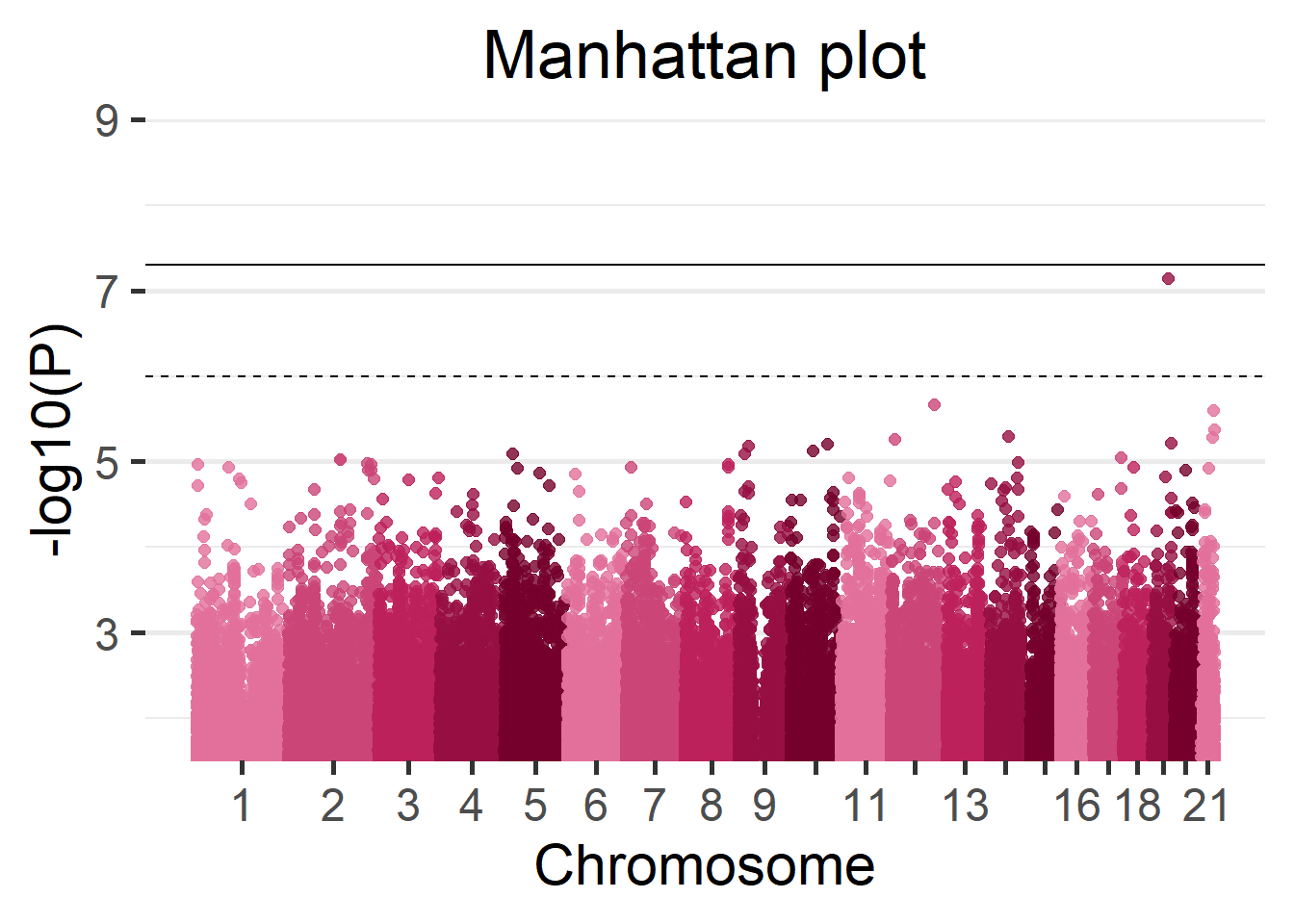
# ... with 865,230 more rowsWe can display the results of the GWAS using a Manhattan plot.
manhattan(results_single)
(#fig:singleCohortManhattan_plot)Manhattan plot of the single-cohort results.
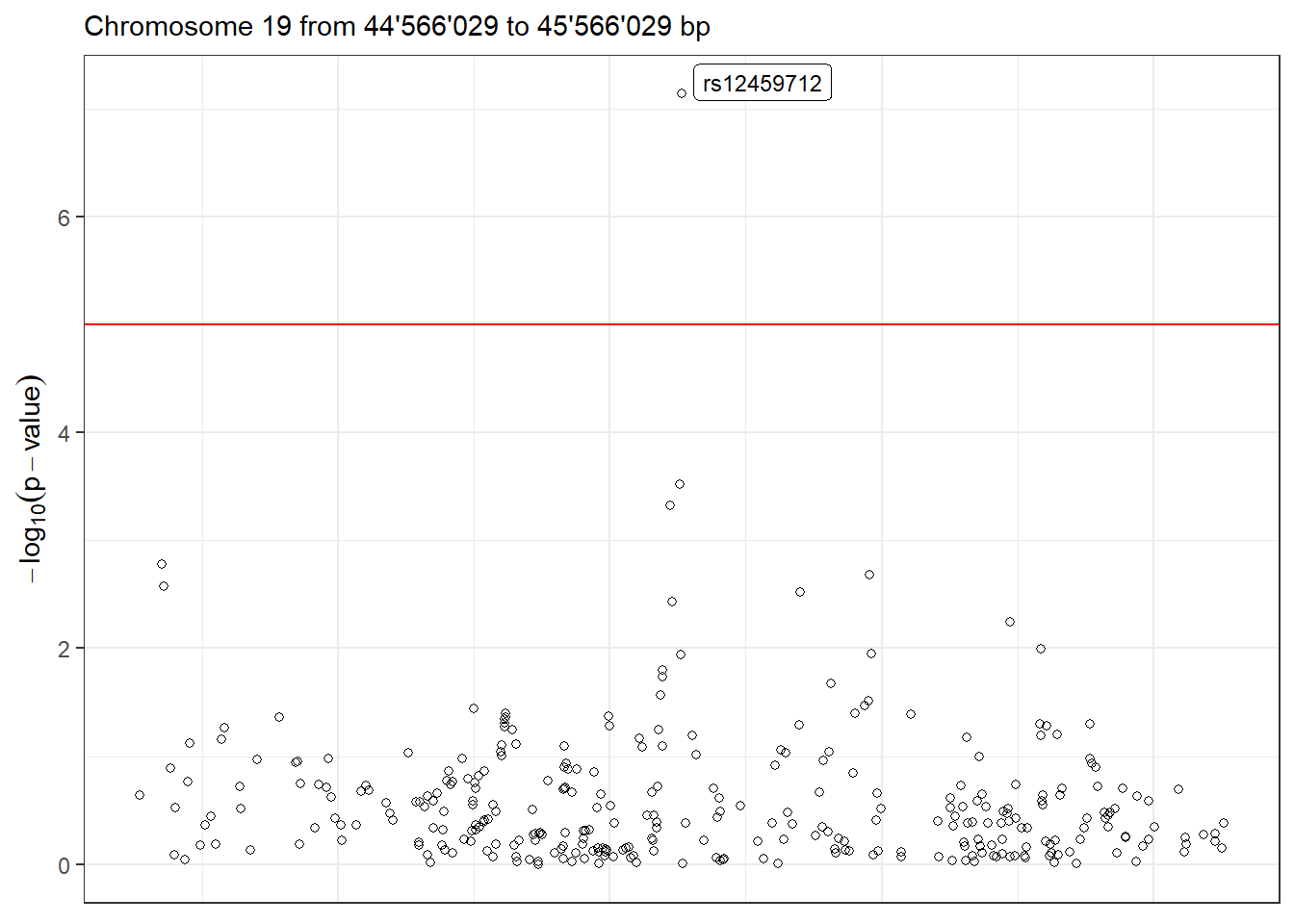
Moreover, we can visualize the region with the lowest p-value in detail using the function LocusZoom. There are multiple arguments to control the gene annotation, display a different region of the GWAS, display a different range of positions and more. Make sure to check ?LocusZoom for all the details.
LocusZoom(results_single, use_biomaRt = FALSE)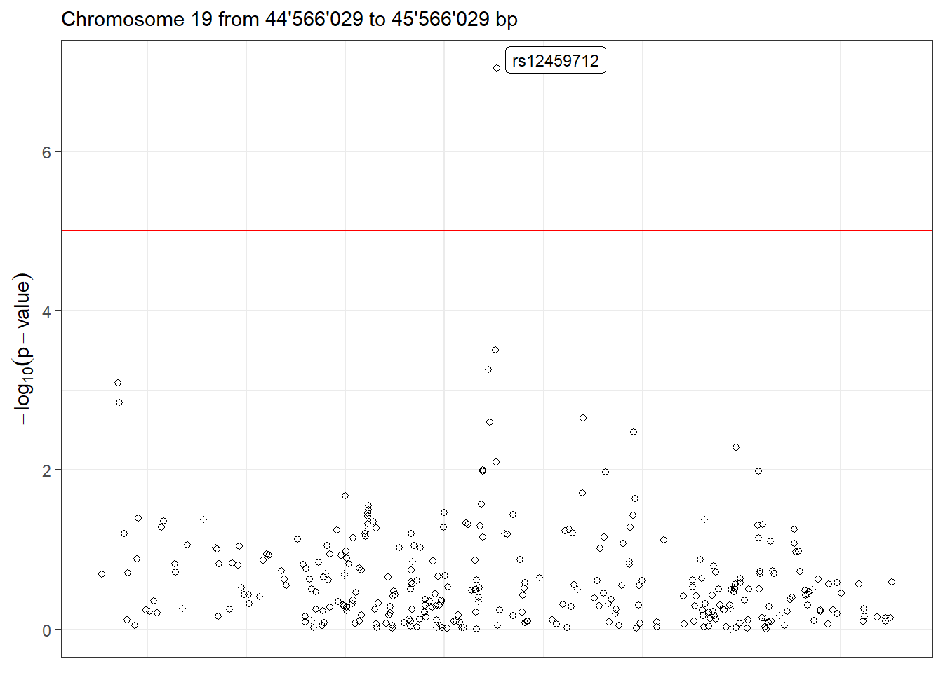
Figure 5.2: LocusZoom plot of the surrounding region of the top hit SNP.
datashield.logout(conns)5.2 Multi cohorts
|
⚠️ RESOURCES USED ALONG THIS SECTION |
|||||||||||||||||||||
|---|---|---|---|---|---|---|---|---|---|---|---|---|---|---|---|---|---|---|---|---|---|
|
From https://opal-demo.obiba.org/ : |
|||||||||||||||||||||
|
Now all the individuals used for the single cohort use case will be divided into three different synthetic cohorts. The results from each cohort will then be meta-analyzed to be compared to the results obtained by studying all the individuals together. As with the single-cohort methodology illustrated on the prior section, this method guarantees GDPR data confidentiality. The structure for a three cohort study is illustrated on the following figure (note this can be extrapolated for cohorts with a bigger (or lower) partner count).
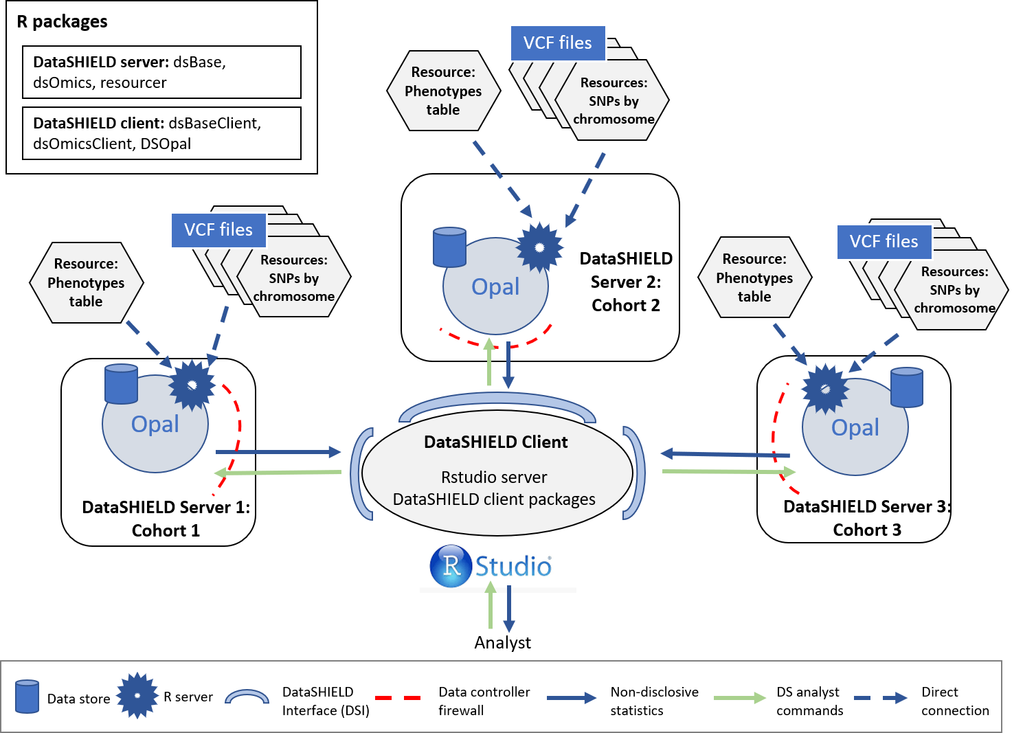
Figure 5.3: Proposed infrastructure to perform multi-cohort GWAS studies.
The data analyst corresponds to the “RStudio” session, which through DataSHIELD Interface (DSI) connects with the Opal server located at the cohort network. This Opal server contains an array of resources that correspond to the different VCF files (sliced by chromosome) 4 and a resource that corresponds to the phenotypes table of the studied individuals.
This use case will portray a complete study methodology, more precisely we will follow this flowchart:
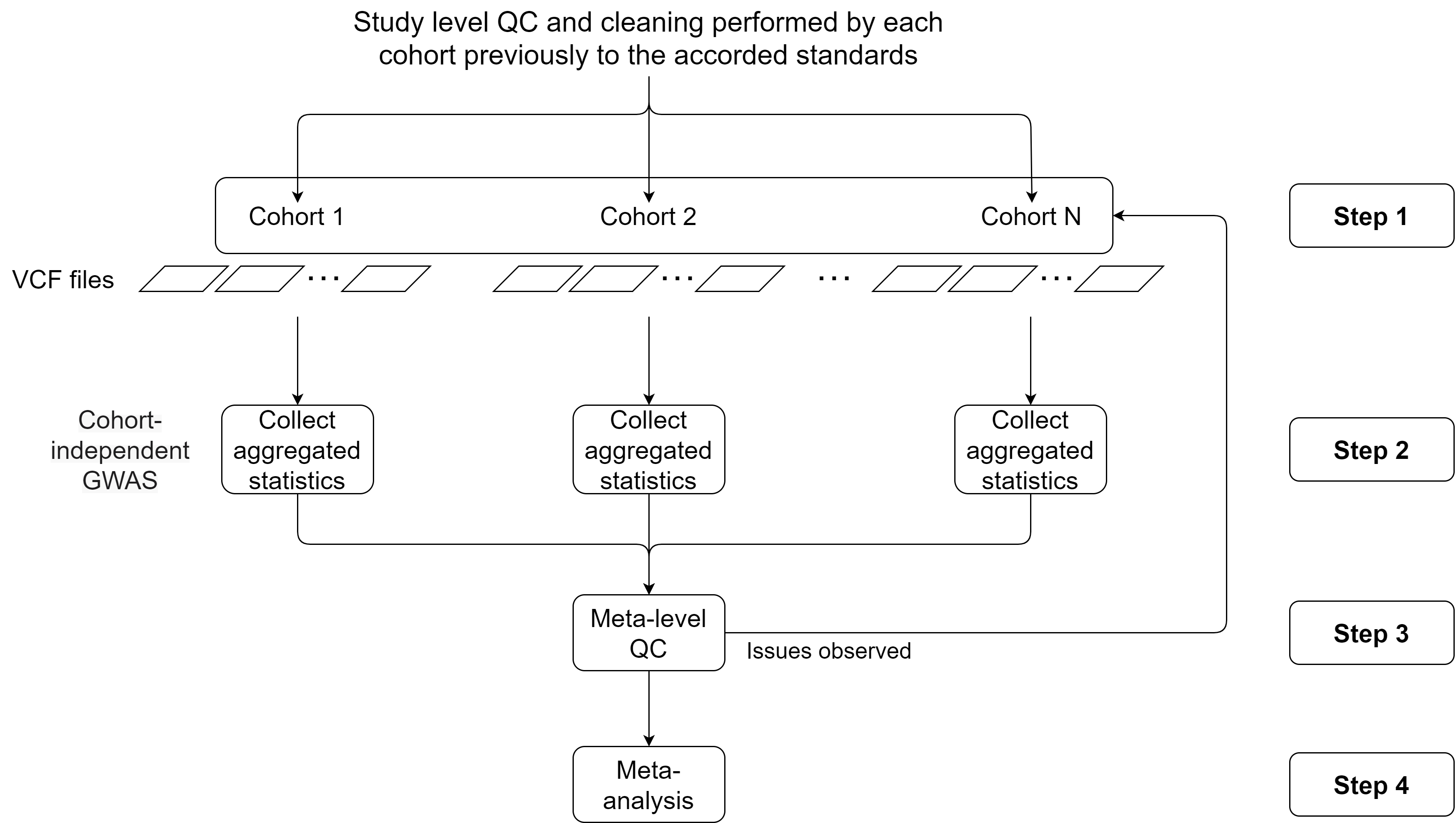
Figure 5.4: Flowchart to perform multi-cohort GWAS studies. Adapted from Winkler et al. (2014)
Brief description of each step:
- Step 1: Logging into the Opal servers and load all the VCF files to the remote R sessions. Corresponds to the sections Connection to the Opal server, Assign the VCF resources, Assign the phenotypes and Merge VCF (genotype) and phenotype information.
- Step 2: Performing a GWAS analysis on each cohort and collect all the aggregated non-disclosive statistics. Corresponds to the sections Performing the GWAS and GWAS Plots.
- Step 3: Apply different QC control methodologies to assess possible problems on the data used on each cohort to perform the analysis. Corresponds to the section Meta-level quality control.
- Step 4: Perform the meta-analysis of the aggregated statistics. Corresponds to the section Meta-analysis.
- Step 5: Perform a pooled ultra fast GWAS and compare the results to the ones of the meta-analysis. Corresponds to the section Ultra fast GWAS.
- Step 6: Perform post-omics analysis: Enrichment analysis. Corresponds to the section Post-omic analysis.
5.2.1 Connection to the Opal server
We have to create an Opal connection object to the different cohorts server. We do that using the following functions.
require('DSI')
require('DSOpal')
require('dsBaseClient')
require('dsOmicsClient')

builder <- DSI::newDSLoginBuilder()
builder$append(server = "cohort1", url = "https://opal-demo.obiba.org/",
               user =  "dsuser", password = "P@ssw0rd",
               driver = "OpalDriver", profile = "omics")
builder$append(server = "cohort2", url = "https://opal-demo.obiba.org/",
               user =  "dsuser", password = "P@ssw0rd",
               driver = "OpalDriver", profile = "omics")
builder$append(server = "cohort3", url = "https://opal-demo.obiba.org/",
               user =  "dsuser", password = "P@ssw0rd",
               driver = "OpalDriver", profile = "omics")
logindata <- builder$build()
conns <- DSI::datashield.login(logins = logindata)
It is important to note that in this use case, we are only using one server that contains all the resources (https://opal-demo.obiba.org/), on this server there are all the resources that correspond to the different cohorts. On a more real scenario each one of the builder$append instructions would be connecting to a different server.
5.2.2 Assign the VCF resources
Now that we have created a connection object to the different Opals, we have started three R session, our analysis will take place on those remote sessions, so we have to load the data into them.
In this use case we will use 63 different resources from the GWAS project hosted on the demo Opal server. This resources correspond to VCF files with information on individual chromosomes (21 chromosomes per three cohorts). The names of the resources are chrXXY (where XX is the chromosome number and Y is the cohort A/B/C). Following the Opal syntax, we will refer to them using the string GWAS.chrXXY.
We have to refer specifically to each different server by using conns[X], this allows us to communicate with the server of interest to indicate to it the resources that it has to load.
# Cohort 1 resources
lapply(1:21, function(x){
  DSI::datashield.assign.resource(conns[1], paste0("chr", x), paste0("GWAS.chr", x,"A"))
  })

# Cohort 2 resources
lapply(1:21, function(x){
  DSI::datashield.assign.resource(conns[2], paste0("chr", x), paste0("GWAS.chr", x,"B"))
  })

# Cohort 3 resources
lapply(1:21, function(x){
  DSI::datashield.assign.resource(conns[3], paste0("chr", x), paste0("GWAS.chr", x,"C"))
  })
Now we have assigned all the resources named GWAS.chrXXY into our remote R session. We have assigned them to the variables called chrXX. To verify this step has been performed correctly, we could use the ds.class function to check for their class and that they exist on the remote sessions.
ds.class("chr1")$cohort1
[1] "GDSFileResourceClient" "FileResourceClient" "ResourceClient"
[4] "R6"
$cohort2
[1] "GDSFileResourceClient" "FileResourceClient" "ResourceClient"
[4] "R6"
$cohort3
[1] "GDSFileResourceClient" "FileResourceClient" "ResourceClient"
[4] "R6" We can see that the object chr1 exists in all the three servers.
Finally the resources are resolved to retrieve the data in the remote sessions.
lapply(1:21, function(x){
  DSI::datashield.assign.expr(conns = conns, symbol = paste0("gds", x, "_object"),
                            expr = as.symbol(paste0("as.resource.object(chr", x, ")")))
})
Now we have resolved the resources named chrXX into our remote R sessions. The objects retrieved have been assigned into variables named gdsXX_object. We can check the process was successful as we did before.
ds.class("gds1_object")$cohort1
[1] "GdsGenotypeReader"
attr(,"package")
[1] "GWASTools"
$cohort2
[1] "GdsGenotypeReader"
attr(,"package")
[1] "GWASTools"
$cohort3
[1] "GdsGenotypeReader"
attr(,"package")
[1] "GWASTools"5.2.3 Assign the phenotypes
The objects we have loaded into our remote sessions are VCF files that contain genomic information of the individuals. To perform a GWAS this information has to be related to some phenotypes to extract relationships. Therefore, we need to load the phenotypes into the remote sessions. The phenotypes information is a table that contains the individuals as rows and phenotypes as columns. In this use case, we will use a resource (as with the VCF files) to load the phenotypes table into the remote sessions.
As with the VCF resources, here we load a different resource to each cohort, as it is expected that each cohort has only the phenotypes information regarding their individuals, therefore different tables. Note that we are assigning the resource to the same variable at each server (pheno), so we only need one function call to resolve all the resources together.
# Cohort 1 phenotypes table
DSI::datashield.assign.resource(conns[1], "pheno", "GWAS.ega_phenotypes_1")

# Cohort 2 phenotypes table
DSI::datashield.assign.resource(conns[2], "pheno", "GWAS.ega_phenotypes_2")

# Cohort 3 phenotypes table
DSI::datashield.assign.resource(conns[3], "pheno", "GWAS.ega_phenotypes_3")

# Resolve phenotypes table
DSI::datashield.assign.expr(conns = conns, symbol = "pheno_object",
                            expr = quote(as.resource.data.frame(pheno)))
We can follow the same analogy as before to know that we have assigned the phenotypes table to a variable called pheno_object on the remote R session.
ds.class("pheno_object")$cohort1
[1] "spec_tbl_df" "tbl_df" "tbl" "data.frame"
$cohort2
[1] "spec_tbl_df" "tbl_df" "tbl" "data.frame"
$cohort3
[1] "spec_tbl_df" "tbl_df" "tbl" "data.frame" We can also check the column names to see which information is present on the table.
ds.colnames("pheno_object")[[1]] [1] "age_cancer_diagnosis" "age_recruitment"
[3] "alcohol_day" "basophill_count"
[5] "behaviour_tumour" "bmi"
[7] "c_reactive_protein_reportability" "record_origin"
[9] "report_format" "cholesterol"
[11] "birth_country" "actual_tobacco_smoker"
[13] "date_diagnosis" "diabetes_diagnosed_doctor"
[15] "diastolic_blood_pressure" "duration_moderate_activity"
[17] "duration_vigorous_activity" "energy"
[19] "eosinophill_count" "ethnicity"
[21] "ever_smoked" "fasting_time"
[23] "alcohol_frequency" "hdl_cholesterol"
[25] "hip_circumference" "histology_tumour"
[27] "home_e_coordinate" "home_n_coordinate"
[29] "e_house_score" "s_house_score"
[31] "w_house_score" "e_income_score"
[33] "w_income_score" "ldl_direct"
[35] "lymphocyte_count" "monocyte_count"
[37] "neutrophill_count" "n_accidental_death_close_gen_family"
[39] "household_count" "children_count"
[41] "operations_count" "operative_procedures"
[43] "past_tobacco" "platelet_count"
[45] "pulse_rate" "qualification"
[47] "cancer_occurrences" "reticulocuyte_count"
[49] "sleep_duration" "height"
[51] "subject_id" "triglycerides"
[53] "cancer_type_idc10" "cancer_type_idc9"
[55] "weight" "leukocyte_count"
[57] "sex" "phenotype"
[59] "age_death" "age_diagnosis_diabetes"
[61] "date_k85_report" "date_k86_report"
[63] "date_death" "enm_diseases"
[65] "source_k85_report" "source_k86_report"
[67] "age_hbp_diagnosis" "mental_disorders"
[69] "respiratory_disorders" "cancer_year"
[71] "circulatory_disorders" "digestive_disorders"
[73] "nervous_disorders" "immune_disorders" 5.2.4 Merge VCF (genotype) and phenotype information
Arrived at this point, we have 21 VCF objects at each cohort R session (each one corresponds to a chromosome) and a phenotypes table. The next step is merging each of the VCF objects with the phenotypes table. The same procedure as the single cohort can be applied to extract the arguments required.
With all this information we can now merge the phenotypes and VCF objects into a type of object named GenotypeData. We will use the ds.GenotypeData function.
lapply(1:21, function(x){
  ds.GenotypeData(x=paste0('gds', x,'_object'), covars = 'pheno_object',
                  columnId = "subject_id", sexId = "sex",
                  male_encoding = "male", female_encoding = "female",
                  case_control_column = "diabetes_diagnosed_doctor",
                  case = "Yes", control = "No",
                  newobj.name = paste0('gds.Data', x), datasources = conns)
})
The objects we just created are named gds.DataXX on the remote session. Now we are ready to perform a GWAS analysis. We will use the same formula as the single cohort use case to be able to compare the results later:
diabetes_diagnosed_doctor ~ sex + hdl_cholesterol5.2.5 Performing a meta - GWAS
We now proceed to perform the GWAS analysis.
results <- ds.metaGWAS(genoData = paste0("gds.Data", 1:21),
                       model = diabetes_diagnosed_doctor ~ sex + hdl_cholesterol)
And we can see the results for each cohort.
⠀
# A tibble: 865,162 x 10
   rs      chr       pos p.value n.obs  freq    Est Est.SE ref_allele alt_allele
 * <chr>   <chr>   <int>   <dbl> <dbl> <dbl>  <dbl>  <dbl> <chr>      <chr>
 1 rs5795~ 1      3.90e7 4.11e-7   430 0.737  0.724  0.143 T          C
 2 rs1132~ 1      1.17e8 5.21e-7   428 0.876 -0.943  0.188 T          C
 3 rs4970~ 1      3.90e7 5.72e-6   350 0.749  0.740  0.163 A          G
 4 rs9726~ 1      2.81e7 7.97e-6   430 0.801  0.695  0.156 C          T
 5 rs2906~ 1      4.43e7 8.97e-6   428 0.551 -0.562  0.127 A          G
 6 rs1211~ 1      1.87e8 6.94e-6   428 0.407 -0.607  0.135 T          A
 7 rs1626~ 1      2.06e8 1.07e-5   428 0.215 -0.693  0.157 C          A
 8 rs1090~ 1      2.81e7 1.04e-5   430 0.8    0.681  0.155 G          A
 9 rs1938~ 1      1.87e8 1.15e-5   429 0.597  0.590  0.134 A          T
10 rs1572~ 1      1.99e7 1.27e-5   428 0.189 -0.739  0.169 T          C
# ... with 865,152 more rows
⠀
# A tibble: 865,190 x 10
   rs      chr       pos p.value n.obs  freq    Est Est.SE ref_allele alt_allele
 * <chr>   <chr>   <int>   <dbl> <dbl> <dbl>  <dbl>  <dbl> <chr>      <chr>
 1 rs9426~ 1      2.98e7 5.14e-6   549 0.756 -0.665  0.146 C          T
 2 rs1240~ 1      8.57e7 8.87e-5   549 0.934  0.918  0.234 A          G
 3 rs2762~ 1      1.45e8 1.10e-4   550 0.52   1.18   0.305 T          C
 4 rs1116~ 1      8.58e7 1.81e-4   549 0.779  0.522  0.139 T          C
 5 rs4657~ 1      1.67e8 2.76e-4   552 0.343 -0.414  0.114 G          T
 6 rs2295~ 1      1.60e8 2.94e-4   549 0.906  0.715  0.197 C          A
 7 rs1891~ 1      1.16e8 2.92e-4   550 0.725  0.500  0.138 T          C
 8 rs7768~ 1      2.21e8 3.03e-4   551 0.928 -0.802  0.222 C          G
 9 rs1209~ 1      3.13e7 3.54e-4   551 0.819 -0.548  0.153 C          T
10 rs6670~ 1      1.16e8 4.08e-4   552 0.724  0.487  0.138 T          C
# ... with 865,180 more rows
⠀
# A tibble: 849,560 x 10
   rs      chr       pos p.value n.obs  freq    Est Est.SE ref_allele alt_allele
 * <chr>   <chr>   <int>   <dbl> <dbl> <dbl>  <dbl>  <dbl> <chr>      <chr>
 1 rs4915~ 1      6.22e7 2.72e-5   285 0.593 -0.700  0.167 G          A
 2 rs7544~ 1      6.22e7 2.87e-5   285 0.593 -0.700  0.167 T          C
 3 rs1385~ 1      1.02e8 3.85e-5   286 0.893  1.09   0.264 A          G
 4 rs1214~ 1      1.72e8 3.76e-5   285 0.909  1.17   0.283 T          G
 5 rs7521~ 1      1.02e8 4.21e-5   285 0.893  1.08   0.264 G          A
 6 rs1337~ 1      1.02e8 4.24e-5   285 0.893  1.08   0.264 A          G
 7 rs6005~ 1      2.45e8 7.08e-5   286 0.893  1.08   0.271 T          A
 8 rs1938~ 1      1.87e8 8.66e-5   285 0.760 -0.743  0.189 C          G
 9 rs1213~ 1      1.72e8 8.36e-5   285 0.919  1.16   0.295 G          T
10 rs7616~ 1      1.72e8 7.93e-5   285 0.919  1.16   0.295 G          C
# ... with 849,550 more rows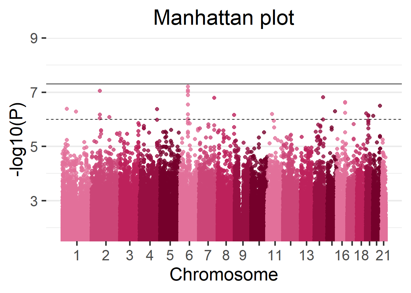
5.2.7 Meta-level quality control
Up to this point we have collected the aggregated statistics from each cohort and we have visualized them. Before meta-analyzing this statistics we have to perform some quality control to make sure there are no major issues. There are three different methods bundled in dsOmicsClient to perform such task:
- EAF Plot: Plotting the reported EAFs against a reference set, such as from the HapMap or 1000 Genomes projects, or from one specific study, can help visualize patterns that pinpoint strand issues, allele miscoding or the inclusion of individuals whose self-reported ancestry did not match their genetic ancestry.
- P-Z Plot: Plot to reveal issues with beta estimates, standard errors and P values. The plots compare P values reported in the association GWAS with P values calculated from Z-statistics (P.ztest) derived from the reported beta and standard error. A study with no issues should show perfect concordance. It will generate a plot per study, where concordance of all the study SNPs will be displayed.
- SE-N Plot: Plot to reveal issues with trait transformations. A collection of studies with no issues will fall on a line.
If any of these QC raises some inconsistencies, please contact the correspondent study analyst.
5.2.7.1 EAF Plot
For this plot we are comparing the estimated allele frequencies to a reference set, so the first step is to get ourselves a reference set. For this example we will be using the ALL.wgs.phase1_release_v3.20101123 reference set. We will download it and load it into the client R session.
reference <- readr::read_tsv("https://homepages.uni-regensburg.de/~wit59712/easyqc/exomechip/ALL.wgs.phase1_release_v3.20101123.snps_indels_sv.sites.EUR_AF.txt.exm.tab.sexChr.DI.txt.GZ")
reference
# A tibble: 75,292 x 8
ExmName chrChr_Pos Chr Pos Rs Ref Alt Freq
<chr> <chr> <dbl> <dbl> <chr> <chr> <chr> <dbl>
1 exm2268640 chr1:762320 1 762320 rs75333668 C T 0.0013
2 exm47 chr1:865628 1 865628 rs41285790 G A 0.01
3 exm55 chr1:865694 1 865694 rs9988179 C T 0.0026
4 exm67 chr1:871159 1 871159 . G A 0.0013
5 exm106 chr1:874762 1 874762 rs139437968 C T 0.0013
6 exm158 chr1:878744 1 878744 . G C 0.0026
7 exm241 chr1:880502 1 880502 rs74047418 C T 0.0013
8 exm2253575 chr1:881627 1 881627 rs2272757 G A 0.63
9 exm269 chr1:881918 1 881918 rs35471880 G A 0.06
10 exm340 chr1:888659 1 888659 rs3748597 T C 0.95
# ... with 75,282 more rowsNow we just use the function eafPlot and we pass to it the GWAS results and the reference set.
eafPlot(x = results, reference = reference, rs_reference = "Rs", freq_reference = "Freq")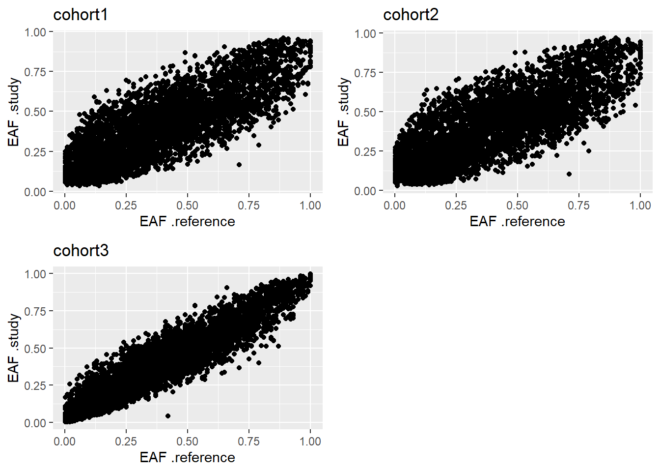
Figure 5.8: EAF Plot.
The obtained results are the expected, which is a linear correlation of slope one. This indicates the alleles are correctly encoded. For further explanation on how to assess the results produced by this plot, please refer to the Figure 4 of Winkler et al. (2014).
5.2.7.2 P-Z Plot
This plot will assess the issues with beta estimates, standard errors and P values. Here we will only need the results from the ds.GWAS function and pass them to the function pzPlot.
pzPlot(results)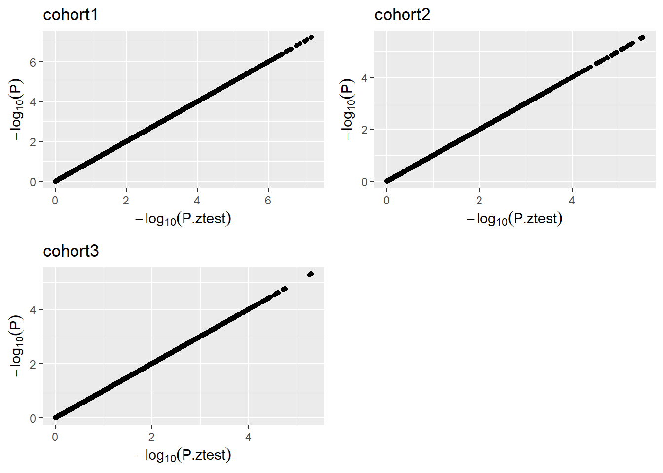
Figure 5.9: P-Z Plot.
Please note that all the SNPs are plotted, for that reason there may be some performance issues if there are many SNPs to be plotted.
A dataset with no issues will show perfect concordance. For further details please refer to the Figure 3 of Winkler et al. (2014).
5.2.7.3 SE-N Plot
Finally, we will assess issues with trait transformations. For this we will only need the results from the ds.GWAS function and pass them to the function seNPlot.
seNPlot(results)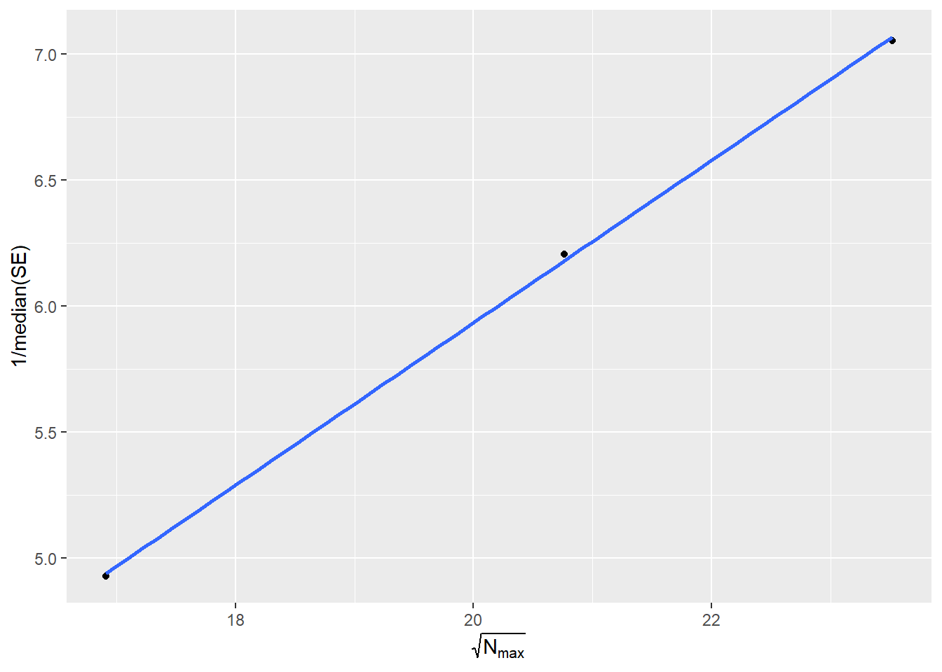
Figure 5.10: SE-N Plot.
If all the study points fall on a line, no issues are present. For further detail please refer to the Figure 2 of Winkler et al. (2014).
5.2.8 Meta-analysis
Given no problems have been detected on the meta-level QC, we will proceed. Up to this point, we have obtained association results for each cohort on the study. The next step is to combine this information using meta-analysis methods to derive a pooled estimate. Each researcher might have an already built pipeline to do so, or a preferred method; nevertheless, we included a couple methods inside dsOmicsClient. They are the following:
- Meta-analysis of p-values: Using the sum of logs method (Fisher’s method).
- Meta-analysis of beta values: Using a fixed-effects model. Methodology extracted and adapted from Pirinen (2020).
5.2.8.1 Assessment of the meta-analysis methods
Previously, we have calculated the same GWAS analysis both using all the individuals and a simulated three-cohort scenario. This gives us the ability to assess how good or bad are the different meta-analysis methods; to do so, we will compare both meta-analysis to the complete data, the evaluation method will be counting the number of top hits that match, more specifically we will search for matches on the top twenty hits.
We apply both methods to the multi-cohort use case results:
meta_pvalues <- metaPvalues(results)
meta_bvalues <- metaBetaValues(results)
We can now compare the 20 top hits from the complete data (previously stored on the variable results_single) to the 20 top hits yielded by both meta-analysis methodologies.
# Extract 20 top hits for all three cases
  # All individuals
top_20_complete <- results_single %>% arrange(p.value) %>% head(20)
  # Pvalue meta-analysis
top_20_pval <- meta_pvalues %>% arrange(p.meta) %>% head(20)
  # Beta meta-analysis
top_20_beta <- meta_bvalues %>% arrange(pval) %>% head(20)

# Number of hits shared by all individuals case and beta meta-analysis
sum(top_20_complete$rs %in% top_20_beta$rs)
[1] 13# Number of hits shared by all individuals case and pvalue meta-analysis
sum(top_20_complete$rs %in% top_20_pval$rs)[1] 1The meta-analysis using beta values recovers a higher amount of top SNPs, therefore it can be considerate a more powerful method for GWAS meta-analyses.
5.2.8.2 Visualizing the results of the meta-analysis
We can use the manhattan plot and locus zoom to visualize the results of the meta-analysis as we visualized the single cohorts before. To help assess the meta-analysis behaviour, we will plot together the meta-analysis results and the complete data results.

5.2.8.3 Meta-analysis versus pooled linear models
The dsOmicsClient package also bundles a function to fit pooled generalized linear models (GLM) on single (or multiple) SNPs. On this section we will compare the results of the meta-analysis to the pooled GLM models to see which method is more accurate. The meta-analysis method will be the beta values (fixed-effects model).
The study methodology will be similar to the one we just performed. The top 20 hits yielded by the meta-analysis will be selected, those SNPs will be studied using the pooled GLM function. Both results will be compared to the complete data.
We aim to replicate a real scenario with this study, typically there is no access to the complete data (if so there is no point on performing meta-analysis on synthetic multi-cohorts), therefore we simulate the discovery of SNPs of interest via meta-analysis, then we want to assess if studying individually those SNPs using pooled GLM will put us closer to the results yielded by having the complete data.
We have already calculated the top 20 SNPs discovered by the beta meta-analysis.
top_20_beta# A tibble: 20 x 10
rs chr pos b.F se.F p.F OR low up pval
<chr> <chr> <int> <dbl> <dbl> <dbl> <dbl> <dbl> <dbl> <dbl>
1 rs124597~ 19 4.51e7 -0.533 0.0989 7.14e-8 0.587 0.484 0.713 7.14e-8
2 rs956025 12 1.19e8 -0.403 0.0850 2.15e-6 0.668 0.566 0.790 2.15e-6
3 rs8130070 21 4.57e7 0.398 0.0846 2.53e-6 1.49 1.26 1.76 2.53e-6
4 rs8130914 21 4.68e7 -0.881 0.191 4.16e-6 0.414 0.285 0.603 4.16e-6
5 rs177569~ 14 6.92e7 -0.613 0.134 5.06e-6 0.542 0.416 0.705 5.06e-6
6 rs9980256 21 4.24e7 -0.388 0.0852 5.20e-6 0.678 0.574 0.801 5.20e-6
7 rs124233~ 12 1.24e7 0.716 0.158 5.47e-6 2.05 1.50 2.79 5.47e-6
8 rs721891 19 5.23e7 -0.492 0.109 6.04e-6 0.612 0.494 0.757 6.04e-6
9 rs112352~ 10 9.88e7 0.765 0.169 6.24e-6 2.15 1.54 3.00 6.24e-6
10 rs9722322 9 2.79e7 0.347 0.0771 6.59e-6 1.42 1.22 1.65 6.59e-6
11 rs169114~ 10 5.97e7 0.681 0.152 7.54e-6 1.98 1.47 2.66 7.54e-6
12 rs122370~ 9 1.72e7 0.497 0.111 7.99e-6 1.64 1.32 2.05 7.99e-6
13 rs7714862 5 2.39e7 0.376 0.0842 8.02e-6 1.46 1.23 1.72 8.02e-6
14 rs8066656 17 7.65e7 -0.551 0.124 8.98e-6 0.576 0.452 0.735 8.98e-6
15 rs101939~ 2 1.39e8 -0.440 0.0992 9.34e-6 0.644 0.530 0.783 9.34e-6
16 rs101853~ 2 1.39e8 -0.411 0.0927 9.45e-6 0.663 0.553 0.795 9.45e-6
17 rs8015318 14 9.76e7 0.340 0.0771 1.02e-5 1.41 1.21 1.63 1.02e-5
18 rs109323~ 2 2.12e8 -0.393 0.0891 1.03e-5 0.675 0.567 0.804 1.03e-5
19 rs4648446 1 2.89e6 -0.326 0.0742 1.08e-5 0.721 0.624 0.834 1.08e-5
20 rs581815 2 2.25e8 -0.343 0.0779 1.08e-5 0.710 0.609 0.827 1.08e-5Next, we have to fit pooled GLM using the ds.glmSNP function, obviously we have to fit the same model that we did on the GWAS (Diabetes.diagnosed.by.doctor ~ sex + HDL.cholesterol), otherwise the results will not be consistent.
The ds.glmSNP function is an extension of the dsBaseClient::ds.glm function, therefore it offers pooled analysis capabilities and disclosure controls.
Remember that we have the genotype data separated by chromosome, following that we will construct the GLM calls as follows:
s <- lapply(1:nrow(top_20_beta), function(x){
  tryCatch({
    ds.glmSNP(snps.fit = top_20_beta[x, 1],
              model = diabetes_diagnosed_doctor ~ sex + hdl_cholesterol,
              genoData = paste0("gds.Data", top_20_beta[x, 2]))
  }, error = function(w){NULL})
})
# Simple data cleaning and column name changes
ss <- data.frame(do.call(rbind, s))
ss <- ss %>% rownames_to_column("rs")
pooled <- ss %>% dplyr::rename(Est.pooled = Estimate,
                               SE.pooled = Std..Error,
                               pval.pooled = p.value) %>%
  dplyr::select(-c(n, p.adj))
We now extract the results of interest from the meta-analysis and the complete data.
# Get data from all individuals study
original <- results_single %>% dplyr::rename(pval.original = p.value,
                                             Est.original = Est,
                                             SE.original = Est.SE) %>%
  dplyr::select(c(rs, Est.original, SE.original, pval.original))
# Arrange dadta from beta meta-analysis
beta <- top_20_beta %>% dplyr::rename(pval.beta = pval,
                                      Est.beta = b.F,
                                      SE.beta = se.F) %>%
  dplyr::select(c(rs, Est.beta, SE.beta, pval.beta))
# Merge all data on a single table
total <- Reduce(function(x,y){inner_join(x,y, by = "rs")},
                list(original, pooled, beta))
With all the information gathered we can visualize the results on the Table 4.
Table 4: Beta values, standard errors and p-values yielded by the three methods: GWAS of all individuals, meta-analysis of synthetic cohorts, pooled analysis of synthetic cohorts.
| SNP id | Beta | SE | P-Value | ||||||
|---|---|---|---|---|---|---|---|---|---|
| Original | Pooled | Meta | Original | Pooled | Meta | Original | Pooled | Meta | |
| rs4648446 | −0.323 | −0.322 | −0.326 | 0.072 | 0.074 | 0.074 | 7.4 × 10⁻⁶ | 1.4 × 10⁻⁵ | 1.1 × 10⁻⁵ |
| rs10932387 | −0.389 | −0.391 | −0.393 | 0.085 | 0.090 | 0.089 | 5.2 × 10⁻⁶ | 1.2 × 10⁻⁵ | 1.0 × 10⁻⁵ |
| rs10193985 | −0.444 | −0.446 | −0.440 | 0.098 | 0.101 | 0.099 | 5.6 × 10⁻⁶ | 1.1 × 10⁻⁵ | 9.3 × 10⁻⁶ |
| rs10185343 | −0.409 | −0.415 | −0.411 | 0.091 | 0.094 | 0.093 | 7.0 × 10⁻⁶ | 1.1 × 10⁻⁵ | 9.4 × 10⁻⁶ |
| rs581815 | −0.341 | −0.344 | −0.343 | 0.077 | 0.079 | 0.078 | 8.3 × 10⁻⁶ | 1.2 × 10⁻⁵ | 1.1 × 10⁻⁵ |
| rs7714862 | 0.376 | 0.371 | 0.376 | 0.081 | 0.084 | 0.084 | 3.2 × 10⁻⁶ | 1.0 × 10⁻⁵ | 8.0 × 10⁻⁶ |
| rs9722322 | 0.353 | 0.345 | 0.347 | 0.076 | 0.078 | 0.077 | 3.3 × 10⁻⁶ | 9.7 × 10⁻⁶ | 6.6 × 10⁻⁶ |
| rs12237062 | 0.497 | 0.499 | 0.497 | 0.108 | 0.113 | 0.111 | 4.3 × 10⁻⁶ | 1.1 × 10⁻⁵ | 8.0 × 10⁻⁶ |
| rs112352624 | 0.685 | 0.814 | 0.765 | 0.160 | 0.186 | 0.169 | 1.9 × 10⁻⁵ | 1.2 × 10⁻⁵ | 6.2 × 10⁻⁶ |
| rs956025 | −0.406 | −0.405 | −0.403 | 0.083 | 0.086 | 0.085 | 9.4 × 10⁻⁷ | 2.3 × 10⁻⁶ | 2.2 × 10⁻⁶ |
| rs12423318 | 0.722 | 0.729 | 0.716 | 0.154 | 0.166 | 0.158 | 2.8 × 10⁻⁶ | 1.1 × 10⁻⁵ | 5.5 × 10⁻⁶ |
| rs17756914 | −0.622 | −0.639 | −0.613 | 0.133 | 0.141 | 0.134 | 2.7 × 10⁻⁶ | 5.8 × 10⁻⁶ | 5.1 × 10⁻⁶ |
| rs8015318 | 0.327 | 0.341 | 0.340 | 0.076 | 0.078 | 0.077 | 1.6 × 10⁻⁵ | 1.2 × 10⁻⁵ | 1.0 × 10⁻⁵ |
| rs8066656 | −0.549 | −0.565 | −0.551 | 0.123 | 0.131 | 0.124 | 8.2 × 10⁻⁶ | 1.7 × 10⁻⁵ | 9.0 × 10⁻⁶ |
| rs12459712 | −0.512 | −0.528 | −0.533 | 0.096 | 0.101 | 0.099 | 9.0 × 10⁻⁸ | 1.6 × 10⁻⁷ | 7.1 × 10⁻⁸ |
| rs721891 | −0.481 | −0.506 | −0.492 | 0.108 | 0.113 | 0.109 | 8.3 × 10⁻⁶ | 7.7 × 10⁻⁶ | 6.0 × 10⁻⁶ |
| rs8130070 | 0.401 | 0.399 | 0.398 | 0.082 | 0.085 | 0.085 | 1.1 × 10⁻⁶ | 2.8 × 10⁻⁶ | 2.5 × 10⁻⁶ |
| rs9980256 | −0.392 | −0.388 | −0.388 | 0.082 | 0.086 | 0.085 | 2.0 × 10⁻⁶ | 5.9 × 10⁻⁶ | 5.2 × 10⁻⁶ |
| rs8130914 | −0.883 | −1.028 | −0.881 | 0.191 | 0.227 | 0.191 | 3.6 × 10⁻⁶ | 5.7 × 10⁻⁶ | 4.2 × 10⁻⁶ |
Finally, to conclude this study we can compute the bias and mean squared error (code not shown). The results are shown on the Table 5.
Table 5: Mean squared error and bias for the betas from the meta-analysis and pooled analysis compared to the complete data (all individuals).
| MSE | Bias | |
|---|---|---|
| Beta | ||
| Pooled | 2.1 × 10⁻³ | 4.8 × 10⁻³ |
| Meta | 3.9 × 10⁻⁴ | −3.0 × 10⁻³ |
With this results we can conclude that refining the statistics for the SNPs of interest using pooled GLM is advisable. Therefore the recommended flowchart when performing a GWAS using dsOmicsClient+DataSHIELD is the following:
REVISAR ESTOS RESULTADOS
- Perform GWAS with
dsOmicsClient::dsGWAS - Perform meta-analysis on the results with
dsOmicsClient::metaBetaValues - Extract top hits from the meta-analysis.
- Perform pooled GLM on top hits with
dsOmicsClient::ds.glmSNP
5.2.9 Ultra fast pooled GWAS analysis
An alternate methodology to performing a meta analysis is to use the fast GWAS methodology. This method is named after the performance it achieves, however, it does provide further advantages other than computational speed. The main advantage is that it does not compute the results for each cohort to then be meta-analyzed, it actually computes them using a pooled technique that achieves the exact same results when all the individuals are together than when they are separated by cohorts. This is of great importance as there is no need to worry about cohort-imbalance, which is usually a problem in multi-cohort meta-analysis studies. The only downside of this method is that it does not yield the same results of a traditional GWAS analysis pipeline, the inacuraccy of the results however is really low, detailed information about that can be found on the paper that proposes the method.
The performance of the function can be summarized to be ~45 seconds per 1M of SNPs (statistic extracted using 2.5k individuals divided into three study servers). From our test this performance has hold linear up to 10M SNPs, we did not test any further. The graphic for < 1M SNPs can be found on the following figure.
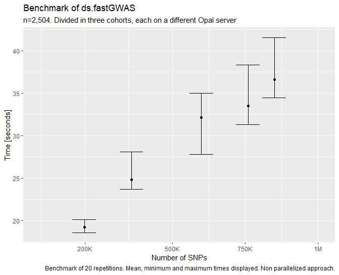
Figure 5.15: Benhmark of ds.fastGWAS function.
The usage is similar to the meta-GWAS with a couple of added options, feel free to check the documentation with ?ds.fastGWAS to see information about them.
results_fast <- ds.fastGWAS(genoData = paste0("gds.Data", 1:21),
                            formula = "diabetes_diagnosed_doctor ~ sex + hdl_cholesterol",
family = "binomial", resample = 6)datashield.logout(conns)5.2.9.1 GWAS Plot
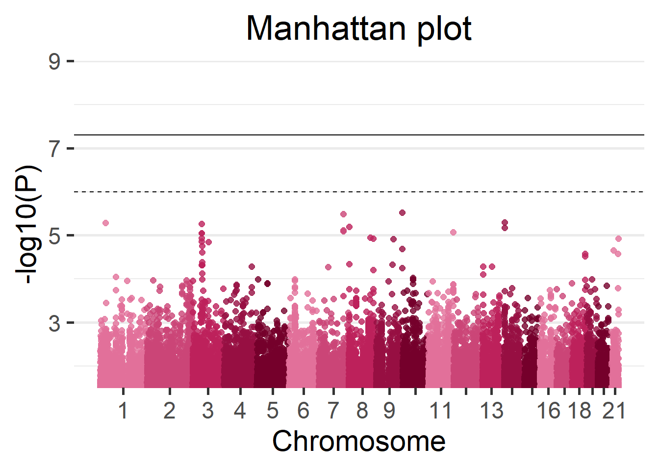
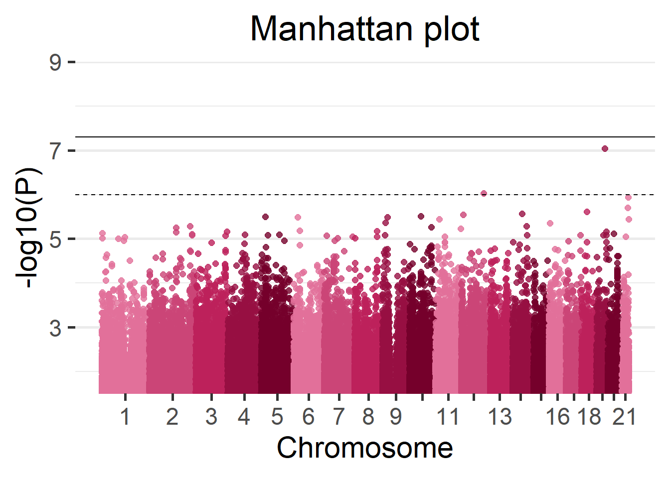
We can display the results of the fast GWAS using a Manhattan plot.
manhattan(results_fast)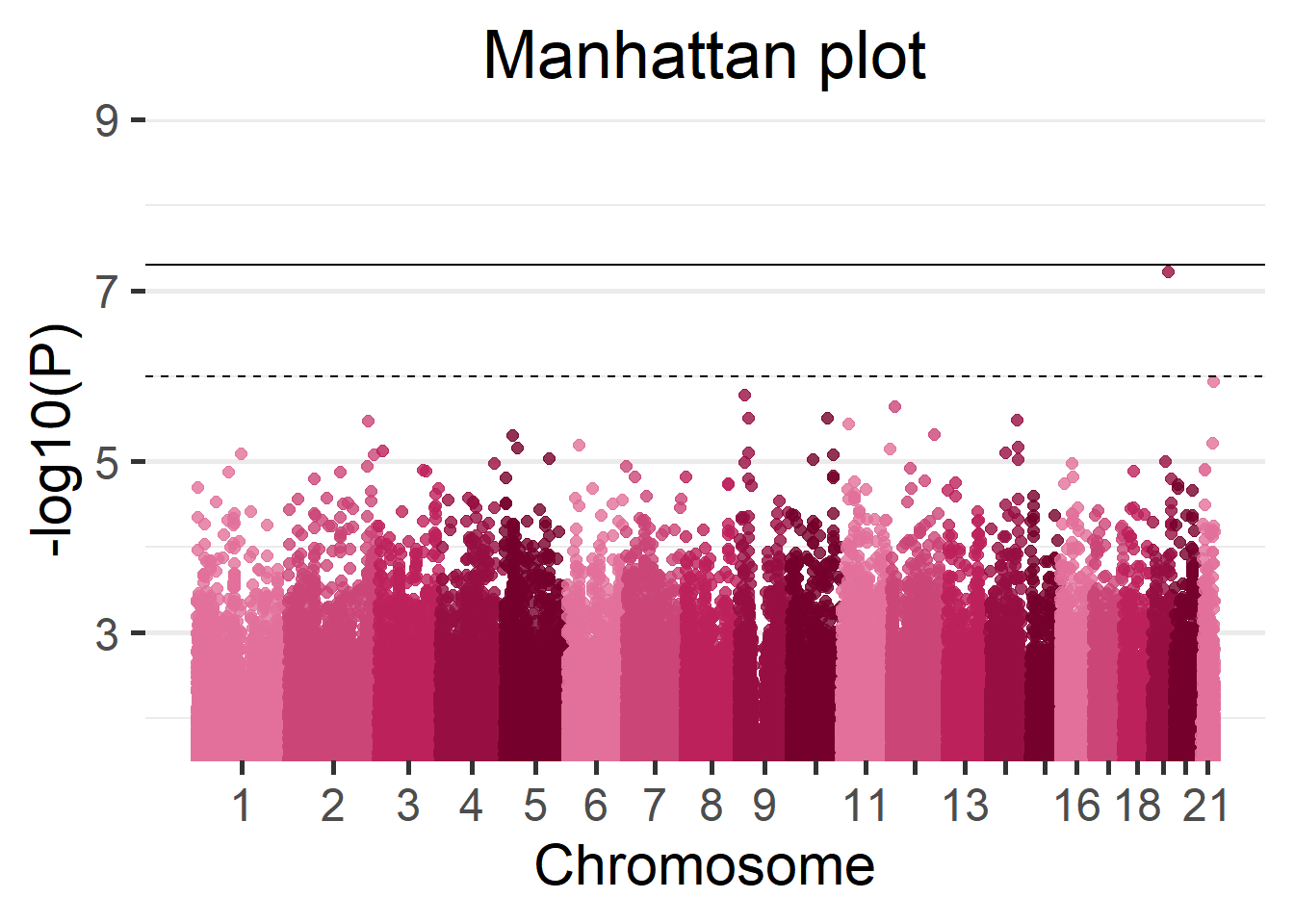
Figure 5.16: Manhattan plot of the Cohort 1.
5.2.9.2 Meta-analysis versus fast GWAS
To finish the GWAS section we can evaluate the results of the beta meta-analysis and the results of the fast GWAS. Both methods will be compared to the ground truth.
As before we can start by seeing the amount of SNPs that both methodologies recover as top hits.
# Extract 20 top hits for all three cases
  # All individuals
top_20_complete <- results_single %>% arrange(p.value) %>% head(20)
  # Fast GWAS
top_20_fast <- results_fast %>% arrange(p.value) %>% head(20)
  # Beta meta-analysis
top_20_beta <- meta_bvalues %>% arrange(pval) %>% head(20)

# Number of hits shared by all individuals case and beta meta-analysis
sum(top_20_complete$rs %in% top_20_beta$rs)
[1] 13# Number of hits shared by all individuals case and fast GWAS
sum(top_20_complete$rs %in% top_20_fast$rs)[1] 11On that regard it seems the meta-analysis is performing better.
We now extract the results of interest from the meta-analysis and the complete data.
# Get data from all individuals study
original <- results_single %>% dplyr::rename(pval.original = p.value,
                                             Est.original = Est,
                                             SE.original = Est.SE) %>%
  dplyr::select(c(rs, Est.original, SE.original, pval.original))
# Arrange dadta from beta meta-analysis
beta <- top_20_beta %>% dplyr::rename(pval.beta = pval,
                                      Est.beta = b.F,
                                      SE.beta = se.F) %>%
  dplyr::select(c(rs, Est.beta, SE.beta, pval.beta))
# Arrange data from fast GWAS
fast <- top_20_fast %>% dplyr::rename(pval.fast = p.value,
                                      Est.fast = Est,
                                      SE.fast = Est.SE) %>%
  dplyr::select(c(rs, Est.fast, SE.fast, pval.fast))
# Merge all data on a single table
total <- Reduce(function(x,y){inner_join(x,y, by = "rs")},
                list(original, fast, beta))
With all the information gathered we can visualize the results on the Table 6.
Table 6: Beta values, standard errors and p-values yielded by the three methods: GWAS of all individuals, meta-analysis of synthetic cohorts, fast GWAS.
| SNP id | Beta | SE | P-Value | ||||||
|---|---|---|---|---|---|---|---|---|---|
| Original | Fast | Meta | Original | Fast | Meta | Original | Fast | Meta | |
| rs7714862 | 0.376 | 0.374 | 0.376 | 0.081 | 0.082 | 0.084 | 3.2 × 10⁻⁶ | 5.0 × 10⁻⁶ | 8.0 × 10⁻⁶ |
| rs9722322 | 0.353 | 0.354 | 0.347 | 0.076 | 0.076 | 0.077 | 3.3 × 10⁻⁶ | 3.1 × 10⁻⁶ | 6.6 × 10⁻⁶ |
| rs12237062 | 0.497 | 0.507 | 0.497 | 0.108 | 0.106 | 0.111 | 4.3 × 10⁻⁶ | 1.7 × 10⁻⁶ | 8.0 × 10⁻⁶ |
| rs112352624 | 0.685 | 0.723 | 0.765 | 0.160 | 0.155 | 0.169 | 1.9 × 10⁻⁵ | 3.1 × 10⁻⁶ | 6.2 × 10⁻⁶ |
| rs956025 | −0.406 | −0.375 | −0.403 | 0.083 | 0.082 | 0.085 | 9.4 × 10⁻⁷ | 4.7 × 10⁻⁶ | 2.2 × 10⁻⁶ |
| rs12423318 | 0.722 | 0.697 | 0.716 | 0.154 | 0.147 | 0.158 | 2.8 × 10⁻⁶ | 2.2 × 10⁻⁶ | 5.5 × 10⁻⁶ |
| rs8015318 | 0.327 | 0.343 | 0.340 | 0.076 | 0.076 | 0.077 | 1.6 × 10⁻⁵ | 6.7 × 10⁻⁶ | 1.0 × 10⁻⁵ |
| rs12459712 | −0.512 | −0.511 | −0.533 | 0.096 | 0.094 | 0.099 | 9.0 × 10⁻⁸ | 6.0 × 10⁻⁸ | 7.1 × 10⁻⁸ |
| rs8130070 | 0.401 | 0.401 | 0.398 | 0.082 | 0.082 | 0.085 | 1.1 × 10⁻⁶ | 1.1 × 10⁻⁶ | 2.5 × 10⁻⁶ |
| rs9980256 | −0.392 | −0.377 | −0.388 | 0.082 | 0.083 | 0.085 | 2.0 × 10⁻⁶ | 6.0 × 10⁻⁶ | 5.2 × 10⁻⁶ |
Finally, to conclude this study we can compute the bias and mean squared error (code not shown). The results are shown on the Table 7.
Table 7: Mean squared error and bias for the betas from the meta-analysis and fast GWAS compared to the complete data (all individuals).
| MSE | Bias | |
|---|---|---|
| Beta | ||
| Fast | 3.6 × 10⁻⁴ | −8.6 × 10⁻³ |
| Meta | 7.2 × 10⁻⁴ | −6.6 × 10⁻³ |
On this brief comparison we’ve seen that the fast GWAS retrieves sensibly less SNPs from the ground truth but it has better performance of bias and MSE. It must be noted that the data used for this GWAS examples does not suffer from any cohort imbalance, so the meta-analysis is expected to yield proper results, on a different environment the fast GWAS is expected to exceed the performance of the meta-analysis in a more remarkable manner.
5.3 Post-omic analysis
Up to this point we have analyzed the genotype and phenotype data by performing a genome wide association study. We can further study the yielded results by performing an enrichment analysis.
5.3.1 Enrichment analysis
The GWAS results are a collection of SNPs that displayed a relationship with a given phenotype. Those SNPs may fall inside gene regions, and those genes can be functionally related. Studying this can help researchers understand the underlying biological processes. Those analysis are carried by querying the selected gene to a database, for this example we will be using the DisGeNET database.
5.3.1.1 Annotation of genes
The first step of the enrichment analysis is to annotate the genes that contain the SNPs of interest yielded by the GWAS. There are many ways to perform this step, we propose to use the biomaRt package and retrieve the annotation from the ensembl genome browser.
First we select the SNPs of interest. We have established a p.value threshold to do so.
snps_of_interest <- results_fast %>%
  dplyr::arrange(p.value) %>%
  dplyr::select(chr, pos, rs, p.value) %>%
  dplyr::filter(p.value < 0.00005)
And with this list of SNPs we can move to the annotation.
library(biomaRt)
# Perform ensembl connection
gene.ensembl <- useEnsembl(biomart = "ensembl",
                           dataset = "hsapiens_gene_ensembl", GRCh = 37)
# Query SNP by SNP
genes_interest <- Reduce(rbind, apply(snps_of_interest, 1, function(x){
  result <- getBM(
    attributes = c('entrezgene_id', 'chromosome_name',
                   'ensembl_gene_id', 'start_position',
                   "end_position"),
    filters = c('start', 'end', 'chromosome_name'),
    values = list(start = x[2], end = x[2],
                  chromosome_name = x[1]),
    mart = gene.ensembl)
}))
5.3.1.2 Enrichment analysis query
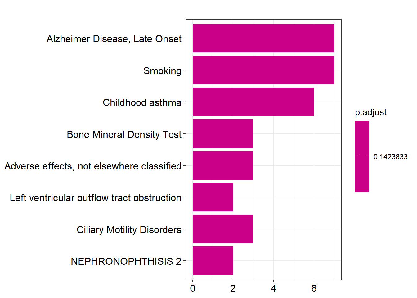
Having the genes of interest annotated, the final step is to query them to DisGeNET. We will use the function enrichDGN from the package DOSE for it. This package is part of a large ecosystem of packages dedicated to enrichment analysis, this allows for easy representation of the query results.
library(DOSE)
enrichment <- enrichDGN(unlist(genes_interest$entrezgene_id),
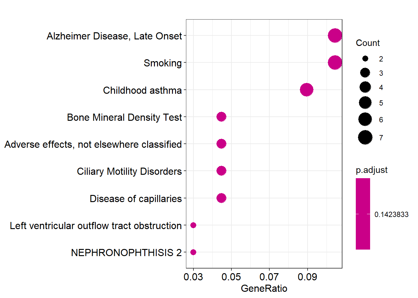
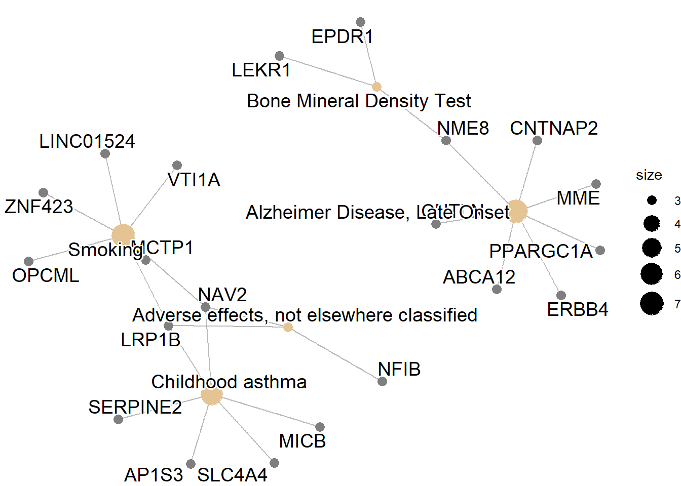
pvalueCutoff = 0.2)5.3.1.3 Enrichment analysis plots
Here we will portray some of the visualizations that can be performed with the query results. For more information and further visualization options please read the official vignette.
References
The same methodology and code can be used with unitary VCF resources that contain the variant information of all chromosomes.↩︎
The same methodology and code can be used with unitary VCF resources that contain the variant information of all chromosomes.↩︎
It’s important to note that all the other encodings present on the case-control column that are not the case or control, will be turned into missings. As an example, if we have
"cancer"/"no cancer"/"no information"/"prefer not to answer"we can specifcycase="cancer",control="no cancer"and all the individuals with"no information"/"prefer not to answer"will be interpreted as missings.↩︎The same methodology and code can be used with unitary VCF resources that contain the variant information of all chromosomes.↩︎