4 Exploration of Genotype data
|
⚠️ RESOURCES USED ALONG THIS SECTION |
|||||||||||||||||||||
|---|---|---|---|---|---|---|---|---|---|---|---|---|---|---|---|---|---|---|---|---|---|
|
From https://opal-demo.obiba.org/ : |
|||||||||||||||||||||
|
Along this section we will illustrate how to get some information about the loaded genotype data and how to perform some basic exploration analysis. Three different aspects will be illustrated:
- Basic information retrieval
- Basic statistics calculation
- Principal component analysis
Information on the data used can be found on the Section (#CINECAopal). We will be working on a virtual scenario with three different cohorts to visualize a real scenario. The same functions can be used in the case of a single cohort.
The study configuration for this section is the following:
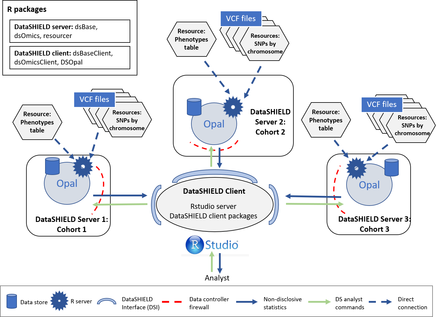
Figure 4.1: Proposed infrastructure.
4.1 Connection to the Opal server
We have to create an Opal connection object to the different cohorts server. We do that using the following functions.
require('DSI')
require('DSOpal')
require('dsBaseClient')
require('dsOmicsClient')

builder <- DSI::newDSLoginBuilder()
builder$append(server = "cohort1", url = "https://opal-demo.obiba.org/",
               user =  "dsuser", password = "P@ssw0rd",
               driver = "OpalDriver", profile = "omics")
builder$append(server = "cohort2", url = "https://opal-demo.obiba.org/",
               user =  "dsuser", password = "P@ssw0rd",
               driver = "OpalDriver", profile = "omics")
builder$append(server = "cohort3", url = "https://opal-demo.obiba.org/",
               user =  "dsuser", password = "P@ssw0rd",
               driver = "OpalDriver", profile = "omics")
logindata <- builder$build()
conns <- DSI::datashield.login(logins = logindata)
It is important to note that in this use case, we are only using one server that contains all the resources (https://opal-demo.obiba.org/), on this server there are all the resources that correspond to the different cohorts. On a more real scenario each one of the builder$append instructions would be connecting to a different server.
4.2 Assign the VCF resources
Now that we have created a connection object to the different Opals, we have started three R session, our analysis will take place on those remote sessions, so we have to load the data into them.
In this use case we will use 63 different resources from the GWAS project hosted on the demo Opal server. This resources correspond to VCF files with information on individual chromosomes (21 chromosomes per three cohorts). The names of the resources are chrXXY (where XX is the chromosome number and Y is the cohort A/B/C). Following the Opal syntax, we will refer to them using the string GWAS.chrXXY.
We have to refer specifically to each different server by using conns[X], this allows us to communicate with the server of interest to indicate to it the resources that it has to load.
# Cohort 1 resources
lapply(1:21, function(x){
  DSI::datashield.assign.resource(conns[1], paste0("chr", x), paste0("GWAS.chr", x,"A"))
  })

# Cohort 2 resources
lapply(1:21, function(x){
  DSI::datashield.assign.resource(conns[2], paste0("chr", x), paste0("GWAS.chr", x,"B"))
  })

# Cohort 3 resources
lapply(1:21, function(x){
  DSI::datashield.assign.resource(conns[3], paste0("chr", x), paste0("GWAS.chr", x,"C"))
  })
Now we have assigned all the resources named GWAS.chrXXY into our remote R session. We have assigned them to the variables called chrXX. To verify this step has been performed correctly, we could use the ds.class function to check for their class and that they exist on the remote sessions.
ds.class("chr1")$cohort1
[1] "GDSFileResourceClient" "FileResourceClient" "ResourceClient"
[4] "R6"
$cohort2
[1] "GDSFileResourceClient" "FileResourceClient" "ResourceClient"
[4] "R6"
$cohort3
[1] "GDSFileResourceClient" "FileResourceClient" "ResourceClient"
[4] "R6" We can see that the object chr1 exists in all the three servers.
Finally the resources are resolved to retrieve the data in the remote sessions.
lapply(1:21, function(x){
  DSI::datashield.assign.expr(conns = conns, symbol = paste0("gds", x, "_object"),
                            expr = as.symbol(paste0("as.resource.object(chr", x, ")")))
})
Now we have resolved the resources named chrXX into our remote R sessions. The objects retrieved have been assigned into variables named gdsXX_object. We can check the process was successful as we did before.
ds.class("gds1_object")$cohort1
[1] "GdsGenotypeReader"
attr(,"package")
[1] "GWASTools"
$cohort2
[1] "GdsGenotypeReader"
attr(,"package")
[1] "GWASTools"
$cohort3
[1] "GdsGenotypeReader"
attr(,"package")
[1] "GWASTools"4.3 Assign the phenotypes
The objects we have loaded into our remote sessions are VCF files that contain genomic information of the individuals. To perform a GWAS this information has to be related to some phenotypes to extract relationships. Therefore, we need to load the phenotypes into the remote sessions. The phenotypes information is a table that contains the individuals as rows and phenotypes as columns. In this use case, we will use a resource (as with the VCF files) to load the phenotypes table into the remote sessions.
As with the VCF resources, here we load a different resource to each cohort, as it is expected that each cohort has only the phenotypes information regarding their individuals, therefore different tables. Note that we are assigning the resource to the same variable at each server (pheno), so we only need one function call to resolve all the resources together.
# Cohort 1 phenotypes table
DSI::datashield.assign.resource(conns[1], "pheno", "GWAS.ega_phenotypes_1")

# Cohort 2 phenotypes table
DSI::datashield.assign.resource(conns[2], "pheno", "GWAS.ega_phenotypes_2")

# Cohort 3 phenotypes table
DSI::datashield.assign.resource(conns[3], "pheno", "GWAS.ega_phenotypes_3")

# Resolve phenotypes table
DSI::datashield.assign.expr(conns = conns, symbol = "pheno_object",
                            expr = quote(as.resource.data.frame(pheno)))
We can follow the same analogy as before to know that we have assigned the phenotypes table to a variable called pheno_object on the remote R session.
ds.class("pheno_object")$cohort1
[1] "spec_tbl_df" "tbl_df" "tbl" "data.frame"
$cohort2
[1] "spec_tbl_df" "tbl_df" "tbl" "data.frame"
$cohort3
[1] "spec_tbl_df" "tbl_df" "tbl" "data.frame" We can also check the column names to see which information is present on the table.
ds.colnames("pheno_object")[[1]] [1] "age_cancer_diagnosis" "age_recruitment"
[3] "alcohol_day" "basophill_count"
[5] "behaviour_tumour" "bmi"
[7] "c_reactive_protein_reportability" "record_origin"
[9] "report_format" "cholesterol"
[11] "birth_country" "actual_tobacco_smoker"
[13] "date_diagnosis" "diabetes_diagnosed_doctor"
[15] "diastolic_blood_pressure" "duration_moderate_activity"
[17] "duration_vigorous_activity" "energy"
[19] "eosinophill_count" "ethnicity"
[21] "ever_smoked" "fasting_time"
[23] "alcohol_frequency" "hdl_cholesterol"
[25] "hip_circumference" "histology_tumour"
[27] "home_e_coordinate" "home_n_coordinate"
[29] "e_house_score" "s_house_score"
[31] "w_house_score" "e_income_score"
[33] "w_income_score" "ldl_direct"
[35] "lymphocyte_count" "monocyte_count"
[37] "neutrophill_count" "n_accidental_death_close_gen_family"
[39] "household_count" "children_count"
[41] "operations_count" "operative_procedures"
[43] "past_tobacco" "platelet_count"
[45] "pulse_rate" "qualification"
[47] "cancer_occurrences" "reticulocuyte_count"
[49] "sleep_duration" "height"
[51] "subject_id" "triglycerides"
[53] "cancer_type_idc10" "cancer_type_idc9"
[55] "weight" "leukocyte_count"
[57] "sex" "phenotype"
[59] "age_death" "age_diagnosis_diabetes"
[61] "date_k85_report" "date_k86_report"
[63] "date_death" "enm_diseases"
[65] "source_k85_report" "source_k86_report"
[67] "age_hbp_diagnosis" "mental_disorders"
[69] "respiratory_disorders" "cancer_year"
[71] "circulatory_disorders" "digestive_disorders"
[73] "nervous_disorders" "immune_disorders" 4.4 Merge VCF (genotype) and phenotype information
Arrived at this point, we have 21 VCF objects at each cohort R session (each one corresponds to a chromosome) and a phenotypes table. The next step is merging each of the VCF objects with the phenotypes table. The same procedure as the single cohort can be applied to extract the arguments required.
With all this information we can now merge the phenotypes and VCF objects into a type of object named GenotypeData. We will use the ds.GenotypeData function.
lapply(1:21, function(x){
  ds.GenotypeData(x=paste0('gds', x,'_object'), covars = 'pheno_object',
                  columnId = "subject_id", sexId = "sex",
                  male_encoding = "male", female_encoding = "female",
                  case_control_column = "diabetes_diagnosed_doctor",
                  case = "Yes", control = "No",
                  newobj.name = paste0('gds.Data', x), datasources = conns)
})
The objects we just created are named gds.DataXX on the remote session. Now we are ready to perform the exploration analysis on the data we just loaded on the remote sessions.
4.5 Basic information of the Genotype data
Once we have everything loaded in the remote R sessions, we can begin a simple exploratory analysis by checking basic information. We can check the following:
- The number of variants, chromosome and individuals
- The available phenotypes (only applies if we have merged phenotypes information)
- Get the available SNP rs IDs
To get the number of variants and individuals:
dimensions <- do.call(rbind, lapply(1:21, function(x){
  data.frame(ds.genoDimensions(paste0('gds.Data', x)))
}))

data.frame(dimensions)
cohort1.snp_number cohort1.scan_number cohort1.chromosomes
1 69806 817 1
2 74985 817 2
3 53164 817 3
4 56259 817 4
5 51985 817 5
6 54835 817 6
7 53037 817 7
8 50372 817 8
9 40920 817 9
10 47075 817 10
11 44979 817 11
12 43477 817 12
13 33411 817 13
14 29742 817 14
15 26905 817 15
16 29183 817 16
17 24546 817 17
18 26353 817 18
19 20408 817 19
20 20771 817 20
21 13079 817 21
cohort2.snp_number cohort2.scan_number cohort2.chromosomes
1 69806 1073 1
2 74985 1073 2
3 53164 1073 3
4 56259 1073 4
5 51985 1073 5
6 54835 1073 6
7 53037 1073 7
8 50372 1073 8
9 40920 1073 9
10 47075 1073 10
11 44979 1073 11
12 43477 1073 12
13 33411 1073 13
14 29742 1073 14
15 26905 1073 15
16 29183 1073 16
17 24546 1073 17
18 26353 1073 18
19 20408 1073 19
20 20771 1073 20
21 13079 1073 21
cohort3.snp_number cohort3.scan_number cohort3.chromosomes
1 69806 557 1
2 74985 557 2
3 53164 557 3
4 56259 557 4
5 51985 557 5
6 54835 557 6
7 53037 557 7
8 50372 557 8
9 40920 557 9
10 47075 557 10
11 44979 557 11
12 43477 557 12
13 33411 557 13
14 29742 557 14
15 26905 557 15
16 29183 557 16
17 24546 557 17
18 26353 557 18
19 20408 557 19
20 20771 557 20
21 13079 557 21To get the available phenotypes:
ds.varLabels('gds.Data1')$cohort1
[1] "age_cancer_diagnosis" "age_recruitment"
[3] "alcohol_day" "basophill_count"
[5] "behaviour_tumour" "bmi"
[7] "c_reactive_protein_reportability" "record_origin"
[9] "report_format" "cholesterol"
[11] "birth_country" "actual_tobacco_smoker"
[13] "date_diagnosis" "diabetes_diagnosed_doctor"
[15] "diastolic_blood_pressure" "duration_moderate_activity"
[17] "duration_vigorous_activity" "energy"
[19] "eosinophill_count" "ethnicity"
[21] "ever_smoked" "fasting_time"
[23] "alcohol_frequency" "hdl_cholesterol"
[25] "hip_circumference" "histology_tumour"
[27] "home_e_coordinate" "home_n_coordinate"
[29] "e_house_score" "s_house_score"
[31] "w_house_score" "e_income_score"
[33] "w_income_score" "ldl_direct"
[35] "lymphocyte_count" "monocyte_count"
[37] "neutrophill_count" "n_accidental_death_close_gen_family"
[39] "household_count" "children_count"
[41] "operations_count" "operative_procedures"
[43] "past_tobacco" "platelet_count"
[45] "pulse_rate" "qualification"
[47] "cancer_occurrences" "reticulocuyte_count"
[49] "sleep_duration" "height"
[51] "scanID" "triglycerides"
[53] "cancer_type_idc10" "cancer_type_idc9"
[55] "weight" "leukocyte_count"
[57] "sex" "phenotype"
[59] "age_death" "age_diagnosis_diabetes"
[61] "date_k85_report" "date_k86_report"
[63] "date_death" "enm_diseases"
[65] "source_k85_report" "source_k86_report"
[67] "age_hbp_diagnosis" "mental_disorders"
[69] "respiratory_disorders" "cancer_year"
[71] "circulatory_disorders" "digestive_disorders"
[73] "nervous_disorders" "immune_disorders"
$cohort2
[1] "age_cancer_diagnosis" "age_recruitment"
[3] "alcohol_day" "basophill_count"
[5] "behaviour_tumour" "bmi"
[7] "c_reactive_protein_reportability" "record_origin"
[9] "report_format" "cholesterol"
[11] "birth_country" "actual_tobacco_smoker"
[13] "date_diagnosis" "diabetes_diagnosed_doctor"
[15] "diastolic_blood_pressure" "duration_moderate_activity"
[17] "duration_vigorous_activity" "energy"
[19] "eosinophill_count" "ethnicity"
[21] "ever_smoked" "fasting_time"
[23] "alcohol_frequency" "hdl_cholesterol"
[25] "hip_circumference" "histology_tumour"
[27] "home_e_coordinate" "home_n_coordinate"
[29] "e_house_score" "s_house_score"
[31] "w_house_score" "e_income_score"
[33] "w_income_score" "ldl_direct"
[35] "lymphocyte_count" "monocyte_count"
[37] "neutrophill_count" "n_accidental_death_close_gen_family"
[39] "household_count" "children_count"
[41] "operations_count" "operative_procedures"
[43] "past_tobacco" "platelet_count"
[45] "pulse_rate" "qualification"
[47] "cancer_occurrences" "reticulocuyte_count"
[49] "sleep_duration" "height"
[51] "scanID" "triglycerides"
[53] "cancer_type_idc10" "cancer_type_idc9"
[55] "weight" "leukocyte_count"
[57] "sex" "phenotype"
[59] "age_death" "age_diagnosis_diabetes"
[61] "date_k85_report" "date_k86_report"
[63] "date_death" "enm_diseases"
[65] "source_k85_report" "source_k86_report"
[67] "age_hbp_diagnosis" "mental_disorders"
[69] "respiratory_disorders" "cancer_year"
[71] "circulatory_disorders" "digestive_disorders"
[73] "nervous_disorders" "immune_disorders"
$cohort3
[1] "age_cancer_diagnosis" "age_recruitment"
[3] "alcohol_day" "basophill_count"
[5] "behaviour_tumour" "bmi"
[7] "c_reactive_protein_reportability" "record_origin"
[9] "report_format" "cholesterol"
[11] "birth_country" "actual_tobacco_smoker"
[13] "date_diagnosis" "diabetes_diagnosed_doctor"
[15] "diastolic_blood_pressure" "duration_moderate_activity"
[17] "duration_vigorous_activity" "energy"
[19] "eosinophill_count" "ethnicity"
[21] "ever_smoked" "fasting_time"
[23] "alcohol_frequency" "hdl_cholesterol"
[25] "hip_circumference" "histology_tumour"
[27] "home_e_coordinate" "home_n_coordinate"
[29] "e_house_score" "s_house_score"
[31] "w_house_score" "e_income_score"
[33] "w_income_score" "ldl_direct"
[35] "lymphocyte_count" "monocyte_count"
[37] "neutrophill_count" "n_accidental_death_close_gen_family"
[39] "household_count" "children_count"
[41] "operations_count" "operative_procedures"
[43] "past_tobacco" "platelet_count"
[45] "pulse_rate" "qualification"
[47] "cancer_occurrences" "reticulocuyte_count"
[49] "sleep_duration" "height"
[51] "scanID" "triglycerides"
[53] "cancer_type_idc10" "cancer_type_idc9"
[55] "weight" "leukocyte_count"
[57] "sex" "phenotype"
[59] "age_death" "age_diagnosis_diabetes"
[61] "date_k85_report" "date_k86_report"
[63] "date_death" "enm_diseases"
[65] "source_k85_report" "source_k86_report"
[67] "age_hbp_diagnosis" "mental_disorders"
[69] "respiratory_disorders" "cancer_year"
[71] "circulatory_disorders" "digestive_disorders"
[73] "nervous_disorders" "immune_disorders"
attr(,"class")
[1] "dsvarLabels" "list" To get the SNP rs IDs:
head(ds.getSNPs('gds.Data1'))[1] "rs575272151" "rs75454623" "rs2691315" "rs2691277" "rs114420996"
[6] "rs62637817" 4.6 Basic statistics of the genotype data
We have also developed functions to compute statistics of the genotype data, the statistics implemented on dsOmicsClient are:
- Allele frequencies. Brief definition (by Nature)[https://www.nature.com/scitable/definition/allele-frequency-298/#:~:text=An%20allele%20frequency%20is%20calculated,a%20percentage%2C%20or%20a%20fraction.].
- Hardy-Weinberg Equilibrium testing. Information on the test can be found (here)[https://www.sciencedirect.com/science/article/pii/S0002929707607356https://www.sciencedirect.com/science/article/pii/S0002929707607356].
To get the allele frequencies we have two different methods, to obtain the pooled frequencies or to obtain them by study server:
# Pooled allele frequencies
ds.alleleFrequency(paste0('gds.Data', 1:21))
# A tibble: 762,900 x 3
rs n pooled_MAF
<chr> <dbl> <dbl>
1 rs575272151 2435 0.0863
2 rs75454623 2428 0.482
3 rs2691315 2429 0.409
4 rs75478250 2432 0.355
5 rs940550 2429 0.297
6 rs144169752 2431 0.120
7 rs368130516 2429 0.0593
8 rs202206030 2433 0.0724
9 rs2853819 2428 0.202
10 rs202025951 2429 0.184
# ... with 762,890 more rows# By-study allele frquencies
ds.alleleFrequency(paste0('gds.Data', 1:21), type = "split")$cohort1
# A tibble: 853,933 x 3
rs n MAF
* <chr> <dbl> <dbl>
1 rs575272151 813 0.0795
2 rs75454623 812 0.476
3 rs2691315 812 0.432
4 rs2691277 813 0.0861
5 rs114420996 812 0.131
6 rs62637817 812 0.0686
7 rs75478250 815 0.348
8 rs940550 812 0.314
9 rs377100675 814 0.259
10 rs62642131 812 0.137
# ... with 853,923 more rows
$cohort2
# A tibble: 855,153 x 3
rs n MAF
* <chr> <dbl> <dbl>
1 rs575272151 1069 0.0965
2 rs75454623 1064 0.491
3 rs2691315 1065 0.433
4 rs2691277 1066 0.0982
5 rs114420996 1064 0.120
6 rs62637817 1064 0.0543
7 rs75478250 1064 0.364
8 rs940550 1065 0.336
9 rs377100675 1066 0.273
10 rs62642131 1063 0.129
# ... with 855,143 more rows
$cohort3
# A tibble: 778,123 x 3
rs n MAF
* <chr> <dbl> <dbl>
1 rs575272151 553 0.0753
2 rs75454623 552 0.477
3 rs2691315 552 0.331
4 rs75478250 553 0.349
5 rs940550 552 0.199
6 rs144169752 553 0.132
7 rs368130516 553 0.0628
8 rs202206030 553 0.0558
9 rs2853819 553 0.236
10 rs202025951 554 0.117
# ... with 778,113 more rows
attr(,"class")
[1] "dsalleleFrequency" "list" To do the Hardy-Weinberg Equilibrium testing is not implemented to get the pooled results as the allele frequency, we can only get the results from each server independently.
do.call(rbind, lapply(1:21, function(x){
  as_tibble(ds.exactHWE(paste0('gds.Data', x)))
}))
# A tibble: 865,292 x 3
cohort1$rs $chr $pval cohort2$rs $chr $pval cohort3$rs $chr
<chr> <chr> <dbl> <chr> <chr> <dbl> <chr> <chr>
1 rs575272151 1 8.10e- 1 rs575272151 1 2.89e- 1 rs575272151 1
2 rs75454623 1 5.90e-115 rs75454623 1 1.22e-160 rs75454623 1
3 rs2691315 1 8.30e- 1 rs2691315 1 3.82e- 1 rs2691315 1
4 rs2691277 1 4.02e- 2 rs2691277 1 2.67e- 3 rs2691277 1
5 rs114420996 1 8.78e- 1 rs114420996 1 1.00e+ 0 rs114420996 1
6 rs62637817 1 2.85e- 5 rs62637817 1 2.94e- 2 rs62637817 1
7 rs75478250 1 4.45e- 2 rs75478250 1 4.27e- 1 rs75478250 1
8 rs940550 1 4.36e- 4 rs940550 1 2.32e- 2 rs940550 1
9 rs377100675 1 5.79e- 43 rs377100675 1 3.34e- 57 rs377100675 1
10 rs62642131 1 4.16e- 5 rs62642131 1 2.01e- 9 rs62642131 1
# ... with 865,282 more rows4.7 Principal component analysis
We have implemented a pooled component analysis method into OmicSHIELD. This function will create new phenotypes on the GenotypeData objects with the principal components results, so we can later adjust our analysis.
pca_res <- ds.PCA(paste0('gds.Data', 1:21), standardize = F)The principal component results can also be visualized using the available grouping variables (categorical) present on the GenotypeData objects used on the ds.PCA function.
dsOmicsClient::plotPCA(pca_res, group = "sex")Or we can visualize the results with no groupings.
dsOmicsClient::plotPCA(pca_res)datashield.logout(conns)