15 Epigenome-wide association analysis (EWAS)
EWAS requires basically the same statistical methods as those used in DGE. It should be notice that the pooled analysis we are going to illustrate here can also be performed with transcriptomic data since each study must have different range values. If so, gene expression harmonization should be performed, for instance, by standardizing the data at each study. For EWAS where methylation is measured using beta values (e.g CpG data are in the range 0-1) this is not a problem. In any case, adopting the meta-analysis approach could be a safe option.
We have downloaded data from GEO corresponding to the accesion number GSE66351 which includes DNA methylation profiling (Illumina 450K array) of 190 individuals. Data corresponds to CpGs beta values measured in the superior temporal gyrus and prefrontal cortex brain regions of patients with Alzheimer’s. Data have been downloaded using GEOquery package that gets GEO data as ExpressionSet objects. Researchers who are not familiar with ExpressionSets can read this Section. Notice that data are encoded as beta-values that ensure data harmonization across studies.
In order to illustrate how to perform data analyses using federated data, we have split the data into two ExpressionSets having 100 and 90 samples as if they were two different studies. Figure 6.2 shows the two resources defined for both studies (GSE66351_1 and GSE66351_2)
In order to perform omic data analyses, we need first to login and assign resources to DataSHIELD. This can be performed using the as.resource.object() function
builder <- DSI::newDSLoginBuilder()
builder$append(server = "study1", url = "https://opal-demo.obiba.org",
               user = "dsuser", password = "password",
               resource = "RSRC.GSE66351_1", driver = "OpalDriver")
builder$append(server = "study2", url = "https://opal-demo.obiba.org",
               user = "dsuser", password = "password",
               resource = "RSRC.GSE66351_2", driver = "OpalDriver")

logindata <- builder$build()

conns <- DSI::datashield.login(logins = logindata, assign = TRUE,
                               symbol = "res")


# Assign to the original R class (e.g ExpressionSet)
datashield.assign.expr(conns, symbol = "methy",
                       expr = quote(as.resource.object(res)))
Now, we can see that the resources are actually loaded into the R servers as their original class
$study1
[1] "ExpressionSet"
attr(,"package")
[1] "Biobase"

$study2
[1] "ExpressionSet"
attr(,"package")
[1] "Biobase"
Then, some Bioconductor-type functions can be use to return non-disclosive information of ExpressionSets from each server to the client, using similar functions as those defined in the dsBaseClient package. For example, feature names can be returned by
$study1
[1] "cg00000029" "cg00000108" "cg00000109" "cg00000165" "cg00000236" "cg00000289"

$study2
[1] "cg00000029" "cg00000108" "cg00000109" "cg00000165" "cg00000236" "cg00000289"
Experimental phenotypes variables can be obtained by
$study1
 [1] "title"                   "geo_accession"           "status"                  "submission_date"
 [5] "last_update_date"        "type"                    "channel_count"           "source_name_ch1"
 [9] "organism_ch1"            "characteristics_ch1"     "characteristics_ch1.1"   "characteristics_ch1.2"
[13] "characteristics_ch1.3"   "characteristics_ch1.4"   "characteristics_ch1.5"   "characteristics_ch1.6"
[17] "characteristics_ch1.7"   "characteristics_ch1.8"   "molecule_ch1"            "extract_protocol_ch1"
[21] "label_ch1"               "label_protocol_ch1"      "taxid_ch1"               "hyb_protocol"
[25] "scan_protocol"           "description"             "data_processing"         "platform_id"
[29] "contact_name"            "contact_email"           "contact_phone"           "contact_laboratory"
[33] "contact_institute"       "contact_address"         "contact_city"            "contact_zip/postal_code"
[37] "contact_country"         "supplementary_file"      "supplementary_file.1"    "data_row_count"
[41] "age"                     "braak_stage"             "brain_region"            "cell type"
[45] "diagnosis"               "donor_id"                "sentrix_id"              "sentrix_position"
[49] "Sex"

$study2
 [1] "title"                   "geo_accession"           "status"                  "submission_date"
 [5] "last_update_date"        "type"                    "channel_count"           "source_name_ch1"
 [9] "organism_ch1"            "characteristics_ch1"     "characteristics_ch1.1"   "characteristics_ch1.2"
[13] "characteristics_ch1.3"   "characteristics_ch1.4"   "characteristics_ch1.5"   "characteristics_ch1.6"
[17] "characteristics_ch1.7"   "characteristics_ch1.8"   "molecule_ch1"            "extract_protocol_ch1"
[21] "label_ch1"               "label_protocol_ch1"      "taxid_ch1"               "hyb_protocol"
[25] "scan_protocol"           "description"             "data_processing"         "platform_id"
[29] "contact_name"            "contact_email"           "contact_phone"           "contact_laboratory"
[33] "contact_institute"       "contact_address"         "contact_city"            "contact_zip/postal_code"
[37] "contact_country"         "supplementary_file"      "supplementary_file.1"    "data_row_count"
[41] "age"                     "braak_stage"             "brain_region"            "cell type"
[45] "diagnosis"               "donor_id"                "sentrix_id"              "sentrix_position"
[49] "Sex"

attr(,"class")
[1] "dsvarLabels" "list"
15.1 Single CpG analysis
Once the methylation data have been loaded into the opal server, we can perform different type of analyses using functions from the dsOmicsClient package. Let us start by illustrating how to analyze a single CpG from two studies by using an approach that is mathematically equivalent to placing all individual-level.
ans <- ds.lmFeature(feature = "cg07363416",
                    model = ~ diagnosis + Sex,
                    Set = "methy",
                    datasources = conns)
ans
Estimate Std. Error p-value
cg07363416 0.03459886 0.02504291 0.1670998
attr(,"class")
[1] "dsLmFeature" "matrix" "array" 15.2 Multiple CpG analysis
The same analysis can be performed for all features (e.g. CpGs) just avoiding the feature argument. This process can be parallelized using mclapply function from the multicore package.
This method corresponds to the pooled analysis approach and can be very time consiming since the function repeatedly calls the DataSHIELD function ds.glm(). We can adopt another strategy that is to run a glm of each feature independently at each study using limma package (which is really fast) and then combine the results (i.e. meta-analysis approach).
Then, we can visualize the top genes at each study (i.e server) by
$study1
# A tibble: 6 x 10
  id           logFC    CI.L    CI.R AveExpr     t       P.Value adj.P.Val     B      SE
  <chr>        <dbl>   <dbl>   <dbl>   <dbl> <dbl>         <dbl>     <dbl> <dbl>   <dbl>
1 cg13138089 -0.147  -0.191  -0.103    0.380 -6.62 0.00000000190  0.000466 10.6  0.0122
2 cg23859635 -0.0569 -0.0741 -0.0397   0.200 -6.58 0.00000000232  0.000466 10.4  0.00520
3 cg13772815 -0.0820 -0.107  -0.0570   0.437 -6.50 0.00000000327  0.000466 10.0  0.0135
4 cg12706938 -0.0519 -0.0678 -0.0359   0.145 -6.45 0.00000000425  0.000466  9.76 0.00872
5 cg24724506 -0.0452 -0.0593 -0.0312   0.139 -6.39 0.00000000547  0.000466  9.51 0.00775
6 cg02812891 -0.125  -0.165  -0.0860   0.247 -6.33 0.00000000731  0.000466  9.23 0.0163

$study2
# A tibble: 6 x 10
  id           logFC    CI.L    CI.R AveExpr     t      P.Value adj.P.Val     B      SE
  <chr>        <dbl>   <dbl>   <dbl>   <dbl> <dbl>        <dbl>     <dbl> <dbl>   <dbl>
1 cg04046629 -0.101  -0.135  -0.0669  0.345  -5.91 0.0000000621    0.0172  7.18 0.0128
2 cg07664323 -0.0431 -0.0577 -0.0284  0.776  -5.85 0.0000000822    0.0172  6.90 0.00390
3 cg27098804 -0.0688 -0.0924 -0.0452  0.277  -5.79 0.000000107     0.0172  6.64 0.0147
4 cg08933615 -0.0461 -0.0627 -0.0296  0.166  -5.55 0.000000298     0.0360  5.64 0.00791
5 cg18349298 -0.0491 -0.0671 -0.0311  0.157  -5.42 0.000000507     0.0489  5.12 0.00848
6 cg02182795 -0.0199 -0.0272 -0.0125  0.0947 -5.36 0.000000670     0.0538  4.84 0.0155
The annotation can be added by using the argument annotCols. It should be a vector with the columns of the annotation available in the ExpressionSet or RangedSummarizedExperiment that want to be showed. The columns of the annotation can be obtained by
$study1
 [1] "ID"                          "Name"                        "AddressA_ID"
 [4] "AlleleA_ProbeSeq"            "AddressB_ID"                 "AlleleB_ProbeSeq"
 [7] "Infinium_Design_Type"        "Next_Base"                   "Color_Channel"
[10] "Forward_Sequence"            "Genome_Build"                "CHR"
[13] "MAPINFO"                     "SourceSeq"                   "Chromosome_36"
[16] "Coordinate_36"               "Strand"                      "Probe_SNPs"
[19] "Probe_SNPs_10"               "Random_Loci"                 "Methyl27_Loci"
[22] "UCSC_RefGene_Name"           "UCSC_RefGene_Accession"      "UCSC_RefGene_Group"
[25] "UCSC_CpG_Islands_Name"       "Relation_to_UCSC_CpG_Island" "Phantom"
[28] "DMR"                         "Enhancer"                    "HMM_Island"
[31] "Regulatory_Feature_Name"     "Regulatory_Feature_Group"    "DHS"
[34] "RANGE_START"                 "RANGE_END"                   "RANGE_GB"
[37] "SPOT_ID"

$study2
 [1] "ID"                          "Name"                        "AddressA_ID"
 [4] "AlleleA_ProbeSeq"            "AddressB_ID"                 "AlleleB_ProbeSeq"
 [7] "Infinium_Design_Type"        "Next_Base"                   "Color_Channel"
[10] "Forward_Sequence"            "Genome_Build"                "CHR"
[13] "MAPINFO"                     "SourceSeq"                   "Chromosome_36"
[16] "Coordinate_36"               "Strand"                      "Probe_SNPs"
[19] "Probe_SNPs_10"               "Random_Loci"                 "Methyl27_Loci"
[22] "UCSC_RefGene_Name"           "UCSC_RefGene_Accession"      "UCSC_RefGene_Group"
[25] "UCSC_CpG_Islands_Name"       "Relation_to_UCSC_CpG_Island" "Phantom"
[28] "DMR"                         "Enhancer"                    "HMM_Island"
[31] "Regulatory_Feature_Name"     "Regulatory_Feature_Group"    "DHS"
[34] "RANGE_START"                 "RANGE_END"                   "RANGE_GB"
[37] "SPOT_ID"

attr(,"class")
[1] "dsfvarLabels" "list"
Then we can run the analysis and obtain the output with the chromosome and gene symbol by:
ans.limma.annot <- ds.limma(model = ~ diagnosis + Sex,
                            Set = "methy",
                            annotCols = c("CHR", "UCSC_RefGene_Name"),
datasources = conns)$study1
# A tibble: 6 x 12
id CHR UCSC_RefGene_Name logFC CI.L CI.R AveExpr t P.Value adj.P.Val B SE
<chr> <chr> <chr> <dbl> <dbl> <dbl> <dbl> <dbl> <dbl> <dbl> <dbl> <dbl>
1 cg131380~ 2 "ECEL1P2" -0.147 -0.191 -0.103 0.380 -6.62 1.90e-9 0.000466 10.6 0.0122
2 cg238596~ 2 "MTA3" -0.0569 -0.0741 -0.0397 0.200 -6.58 2.32e-9 0.000466 10.4 0.00520
3 cg137728~ 17 "" -0.0820 -0.107 -0.0570 0.437 -6.50 3.27e-9 0.000466 10.0 0.0135
4 cg127069~ 19 "MEX3D" -0.0519 -0.0678 -0.0359 0.145 -6.45 4.25e-9 0.000466 9.76 0.00872
5 cg247245~ 19 "ISOC2;ISOC2;ISOC2" -0.0452 -0.0593 -0.0312 0.139 -6.39 5.47e-9 0.000466 9.51 0.00775
6 cg028128~ 2 "ECEL1P2" -0.125 -0.165 -0.0860 0.247 -6.33 7.31e-9 0.000466 9.23 0.0163
$study2
# A tibble: 6 x 12
id CHR UCSC_RefGene_Name logFC CI.L CI.R AveExpr t P.Value adj.P.Val B SE
<chr> <chr> <chr> <dbl> <dbl> <dbl> <dbl> <dbl> <dbl> <dbl> <dbl> <dbl>
1 cg04046629 11 "CD6" -0.101 -0.135 -0.0669 0.345 -5.91 0.0000000621 0.0172 7.18 0.0128
2 cg07664323 6 "MUC21" -0.0431 -0.0577 -0.0284 0.776 -5.85 0.0000000822 0.0172 6.90 0.00390
3 cg27098804 11 "CD6" -0.0688 -0.0924 -0.0452 0.277 -5.79 0.000000107 0.0172 6.64 0.0147
4 cg08933615 1 "" -0.0461 -0.0627 -0.0296 0.166 -5.55 0.000000298 0.0360 5.64 0.00791
5 cg18349298 3 "RARRES1;RARRES1" -0.0491 -0.0671 -0.0311 0.157 -5.42 0.000000507 0.0489 5.12 0.00848
6 cg02182795 8 "" -0.0199 -0.0272 -0.0125 0.0947 -5.36 0.000000670 0.0538 4.84 0.0155 Then, the last step is to meta-analyze the results. Different methods can be used to this end. We have implemented a method that meta-analyze the p-pvalues of each study as follows:
# A tibble: 481,868 x 4
   id                study1      study2   p.meta
   <chr>              <dbl>       <dbl>    <dbl>
 1 cg13138089 0.00000000190 0.00000763  4.78e-13
 2 cg25317941 0.0000000179  0.00000196  1.12e-12
 3 cg02812891 0.00000000731 0.00000707  1.63e-12
 4 cg12706938 0.00000000425 0.0000161   2.14e-12
 5 cg16026647 0.000000101   0.000000797 2.51e-12
 6 cg12695465 0.00000000985 0.0000144   4.33e-12
 7 cg21171625 0.000000146   0.00000225  9.78e-12
 8 cg13772815 0.00000000327 0.000122    1.18e-11
 9 cg00228891 0.000000166   0.00000283  1.38e-11
10 cg21488617 0.0000000186  0.0000299   1.62e-11
# ... with 481,858 more rows
We can verify that the results are pretty similar to those obtained using pooled analyses. Here we compute the association for two of the top-CpGs:
res1 <- ds.lmFeature(feature = "cg13138089",
                     model = ~ diagnosis + Sex,
                     Set = "methy",
                     datasources = conns)
res1
Estimate Std. Error p-value
cg13138089 -0.1373348 0.01712405 1.057482e-15
attr(,"class")
[1] "dsLmFeature" "matrix" "array" res2 <- ds.lmFeature(feature = "cg13772815",
model = ~ diagnosis + Sex,
Set = "methy",
datasources = conns)
res2 Estimate Std. Error p-value
cg13772815 -0.06786137 0.009128915 1.056225e-13
attr(,"class")
[1] "dsLmFeature" "matrix" "array" We can create a QQ-plot by using the function qqplot available in our package.
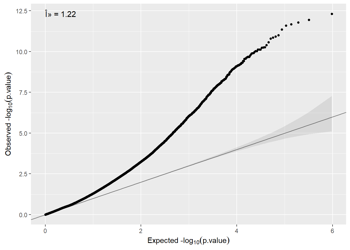
Here In some cases inflation can be observed, so that, correction for cell-type or surrogate variables must be performed. We describe how we can do that in the next two sections.
15.3 Adjusting for Surrogate Variables
The vast majority of omic studies require to control for unwanted variability. The surrogate variable analysis (SVA) can address this issue by estimating some hidden covariates that capture differences across individuals due to some artifacts such as batch effects or sample quality sam among others. The method is implemented in SVA package.
Performing this type of analysis using the ds.lmFeature function is not allowed since estimating SVA would require to implement a non-disclosive method that computes SVA from the different servers. This will be a future topic of the dsOmicsClient. NOTE that, estimating SVA separately at each server would not be a good idea since the aim of SVA is to capture differences mainly due to experimental issues among ALL individuals. What we can do instead is to use the ds.limma function to perform the analyses adjusted for SVA at each study.
ans.sva <- ds.limma(model = ~ diagnosis + Sex,
                    Set = "methy",
                    sva = TRUE, annotCols = c("CHR", "UCSC_RefGene_Name"))
ans.sva
$study1
# A tibble: 481,868 x 12
id CHR UCSC_RefGene_Name logFC CI.L CI.R AveExpr t P.Value adj.P.Val B SE
<chr> <chr> <chr> <dbl> <dbl> <dbl> <dbl> <dbl> <dbl> <dbl> <dbl> <dbl>
1 cg101814~ 19 "GNG7" -0.0547 -0.0721 -0.0373 0.338 -6.25 1.31e-8 0.00591 8.51 0.0103
2 cg137728~ 17 "" -0.0569 -0.0757 -0.0381 0.437 -6.00 3.91e-8 0.00591 7.43 0.00425
3 cg118020~ 19 "PODNL1;PODNL1;POD~ 0.0334 0.0223 0.0445 0.568 5.97 4.53e-8 0.00591 7.29 0.00897
4 cg272310~ 17 "SLC47A2;SLC47A2" 0.0274 0.0182 0.0365 0.548 5.95 4.91e-8 0.00591 7.21 0.00696
5 cg210789~ 6 "" -0.0453 -0.0609 -0.0297 0.799 -5.78 1.05e-7 0.00666 6.46 0.00733
6 cg238596~ 2 "MTA3" -0.0327 -0.0440 -0.0215 0.200 -5.77 1.09e-7 0.00666 6.42 0.0149
7 cg102974~ 16 "SALL1;SALL1" 0.0366 0.0240 0.0492 0.137 5.77 1.10e-7 0.00666 6.42 0.00688
8 cg249245~ 1 "" 0.0317 0.0208 0.0427 0.821 5.76 1.11e-7 0.00666 6.41 0.00969
9 cg136631~ 9 "" -0.0326 -0.0440 -0.0213 0.367 -5.72 1.32e-7 0.00705 6.24 0.00562
10 cg131380~ 2 "ECEL1P2" -0.106 -0.144 -0.0686 0.380 -5.61 2.15e-7 0.00835 5.76 0.00137
# ... with 481,858 more rows
$study2
# A tibble: 481,868 x 12
id CHR UCSC_RefGene_Na~ logFC CI.L CI.R AveExpr t P.Value adj.P.Val B SE
<chr> <chr> <chr> <dbl> <dbl> <dbl> <dbl> <dbl> <dbl> <dbl> <dbl> <dbl>
1 cg16766632 12 "LRP1" -0.0418 -0.0548 -0.0289 0.388 -6.42 7.82e-9 0.00374 9.05 0.00917
2 cg25036710 1 "" -0.0664 -0.0874 -0.0453 0.569 -6.27 1.55e-8 0.00374 8.37 0.00373
3 cg12938128 11 "NRXN2;NRXN2" -0.0273 -0.0367 -0.0179 0.728 -5.81 1.13e-7 0.0149 6.42 0.00901
4 cg07349815 3 "" -0.0393 -0.0529 -0.0258 0.160 -5.78 1.24e-7 0.0149 6.32 0.00737
5 cg07664323 6 "MUC21" -0.0427 -0.0579 -0.0276 0.776 -5.61 2.63e-7 0.0163 5.59 0.00682
6 cg00228891 1 "CR1L" -0.0568 -0.0771 -0.0365 0.350 -5.56 3.18e-7 0.0163 5.40 0.0139
7 cg11743675 12 "CNTN1;CNTN1" -0.0443 -0.0601 -0.0284 0.152 -5.56 3.18e-7 0.0163 5.40 0.00786
8 cg03470754 7 "PGAM2;PGAM2" -0.0442 -0.0600 -0.0283 0.211 -5.56 3.26e-7 0.0163 5.38 0.00790
9 cg07015749 1 "KCNAB2;KCNAB2" 0.0611 0.0392 0.0831 0.659 5.54 3.47e-7 0.0163 5.31 0.00469
10 cg25647784 17 "WNK4" -0.0392 -0.0533 -0.0251 0.512 -5.52 3.70e-7 0.0163 5.25 0.00157
# ... with 481,858 more rows
attr(,"class")
[1] "dsLimma" "list" Then, data can be combined meta-anlyzed as follows:
# A tibble: 481,868 x 4
   id               study1      study2   p.meta
   <chr>             <dbl>       <dbl>    <dbl>
 1 cg00228891 0.00000397   0.000000318 3.58e-11
 2 cg01301319 0.00000609   0.00000123  2.00e-10
 3 cg22962123 0.00000106   0.00000767  2.17e-10
 4 cg24302412 0.0000139    0.000000762 2.77e-10
 5 cg02812891 0.000000408  0.0000327   3.47e-10
 6 cg23859635 0.000000109  0.000190    5.29e-10
 7 cg13138089 0.000000215  0.000105    5.74e-10
 8 cg24938077 0.0000125    0.00000254  8.02e-10
 9 cg13772815 0.0000000391 0.00132     1.27e- 9
10 cg21212881 0.000000340  0.000248    2.04e- 9
# ... with 481,858 more rows
The DataSHIELD session must by closed by: