3 Bioconductor Data Structures
Bioconductor promotes the statistical analysis and comprehension of current and emerging high-throughput biological assays. Bioconductor is based on packages written primarily in the R programming language. Bioconductor is committed to open source, collaborative, distributed software development and literate, reproducible research. Most Bioconductor components are distributed as R packages. The functional scope of Bioconductor packages includes the analysis of DNA microarray, sequence, flow, SNP, and other data.
Bioconductor provides several data infrastructures for efficiently managing omic data. See this paper for a global overview. Here we provide a quick introduction for the most commonly used ones. We also recommend to learn how to deal with GenomicRanges which helps to efficiently manage genomic data information.
3.1 SNP Array Data
SNP array data are normally stored in PLINK format (or VCF for NGS data). PLINK data are normally stored in three files .ped, .bim, .fam. The advantage is that SNP data are stored in binary format in the BED file (Homozygous normal 01, Heterozygous 02, Homozygous variant 03, missing 00).
- FAM file: one row per individual - identification information: Family ID, Individual ID Paternal ID, Maternal ID, Sex (1=male; 2=female; other=unknown), Phenotype.
- BIM file: one row per SNP (rs id, chromosome, position, allele 1, allele 2).
- BED file: one row per individual. Genotypes in columns.
Data are easily loaded into R by using read.plink function
require(snpStats)
snps <- read.plink("data/obesity") # there are three files obesity.fam, obesity.bim, obesity.bed
names(snps)
[1] "genotypes" "fam" "map" Genotypes is a snpMatrix object
A SnpMatrix with  2312 rows and  100000 columns
Row names:  100 ... 998
Col names:  MitoC3993T ... rs28600179
Annotation is a data.frame object
           chromosome   snp.name cM position allele.1 allele.2
MitoC3993T         NA MitoC3993T NA     3993        T        C
MitoG4821A         NA MitoG4821A NA     4821        A        G
MitoG6027A         NA MitoG6027A NA     6027        A        G
MitoT6153C         NA MitoT6153C NA     6153        C        T
MitoC7275T         NA MitoC7275T NA     7275        T        C
MitoT9699C         NA MitoT9699C NA     9699        C        T
3.2 Expression Sets
The ExpressionSet is a fundamental data container in Bioconductor
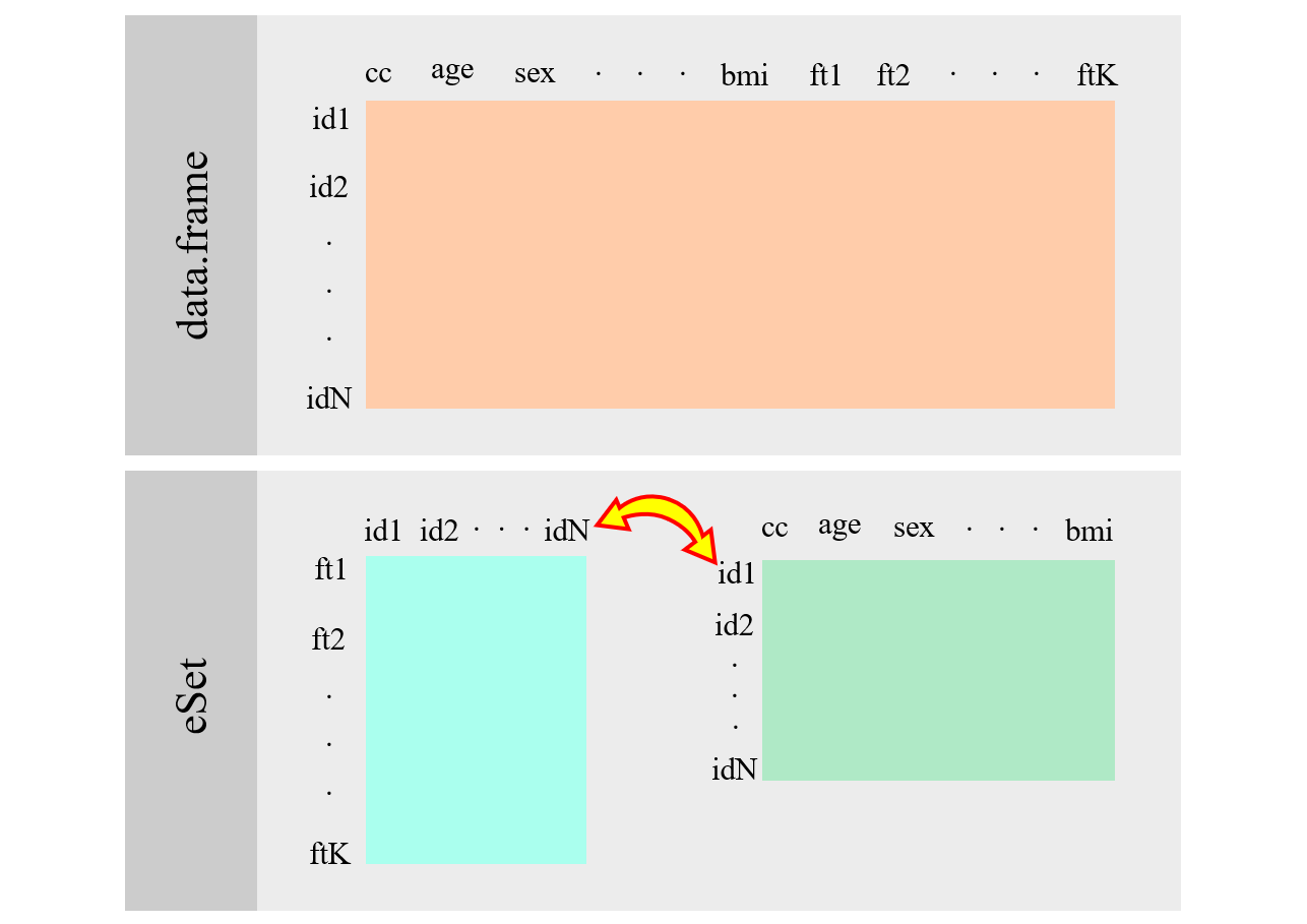
Alt ExpressionSet
Description
Biobaseis part of the Bioconductor project and contains standardized data structures to represent genomic data.The
ExpressionSetclass is designed to combine several different sources of information into a single convenient structure.An
ExpressionSetcan be manipulated (e.g., subsetted, copied) conveniently, and is the input or output from many Bioconductor functions.The data in an
ExpressionSetconsists of expression data from microarray experiments, `meta-data’ describing samples in the experiment, annotations and meta-data about the features on the chip and information related to the protocol used for processing each samplePrint
ExpressionSet (storageMode: lockedEnvironment)
assayData: 52580 features, 69 samples
  element names: exprs
protocolData: none
phenoData
  sampleNames: NA18486 NA18498 ... NA19257 (69 total)
  varLabels: num.tech.reps population study gender
  varMetadata: labelDescription
featureData
  featureNames: ENSG00000000003 ENSG00000000005 ... LRG_99 (52580 total)
  fvarLabels: gene
  fvarMetadata: labelDescription
experimentData: use 'experimentData(object)'
Annotation: - Get experimental data (e.g., gene expression)
                NA18486 NA18498 NA18499 NA18501
ENSG00000000003       0       0       0       0
ENSG00000000005       0       0       0       0
ENSG00000000419      22     105      40      55
ENSG00000000457      22     100     107      53
Get phenotypic data (e.g. covariates, disease status, outcomes, …)
        num.tech.reps population    study gender
NA18486             2        YRI Pickrell   male
NA18498             2        YRI Pickrell   male
NA18499             2        YRI Pickrell female
NA18501             2        YRI Pickrell   male
NA18502             2        YRI Pickrell female
NA18504 2 YRI Pickrell male [1] male male female male female male female male female male female male female male female
[16] male female female male female male female female male female male female female male female
[31] female male female male female female female female male female male male female female male
[46] female female male female female male female male male female female male female male female
[61] male female female male female female female male female
Levels: female maleThis also works
 [1] male   male   female male   female male   female male   female male   female male   female male   female
[16] male   female female male   female male   female female male   female male   female female male   female
[31] female male   female male   female female female female male   female male   male   female female male
[46] female female male   female female male   female male   male   female female male   female male   female
[61] male   female female male   female female female male   female
Levels: female maleSubsetting (everything is synchronized)
ExpressionSet (storageMode: lockedEnvironment)
assayData: 52580 features, 29 samples
  element names: exprs
protocolData: none
phenoData
  sampleNames: NA18486 NA18498 ... NA19239 (29 total)
  varLabels: num.tech.reps population study gender
  varMetadata: labelDescription
featureData
  featureNames: ENSG00000000003 ENSG00000000005 ... LRG_99 (52580 total)
  fvarLabels: gene
  fvarMetadata: labelDescription
experimentData: use 'experimentData(object)'
Annotation:
Finally, the fData function gets the probes’ annotation in a data.frame. Let us first illustrate how to provide an annotation to an ExpressionSet object
require(Homo.sapiens)
geneSymbols <- rownames(genes)
annot <- select(Homo.sapiens, geneSymbols,
                columns=c("TXCHROM", "SYMBOL"), keytype="ENSEMBL")
annotation(pickrell.eset) <- "Homo.sapiens"
fData(pickrell.eset) <- annot
pickrell.eset
ExpressionSet (storageMode: lockedEnvironment)
assayData: 52580 features, 69 samples
element names: exprs
protocolData: none
phenoData
sampleNames: NA18486 NA18498 ... NA19257 (69 total)
varLabels: num.tech.reps population study gender
varMetadata: labelDescription
featureData
featureNames: 1 2 ... 59351 (59351 total)
fvarLabels: ENSEMBL SYMBOL TXCHROM
fvarMetadata: labelDescription
experimentData: use 'experimentData(object)'
Annotation: Homo.sapiens ENSEMBL SYMBOL TXCHROM
1 ENSG00000000003 TSPAN6 chrX
2 ENSG00000000005 TNMD chrX
3 ENSG00000000419 DPM1 chr20
4 ENSG00000000457 SCYL3 chr1
5 ENSG00000000460 C1orf112 chr1
6 ENSG00000000938 FGR chr13.3 Genomic Ranges
The GenomicRanges package serves as the foundation for representing genomic locations within the Bioconductor project.
GRanges(): genomic coordinates to represent annotations (exons, genes, regulatory marks, …) and data (called peaks, variants, aligned reads)GRangesList(): genomic coordinates grouped into list elements (e.g., paired-end reads; exons grouped by transcript)
Operations
- intra-range: act on each range independently
- e.g.,
shift()
- e.g.,
- inter-range: act on all ranges in a
GRangesobject orGRangesListelement - e.g.,reduce();disjoin() - between-range: act on two separate
GRangesorGRangesListobjects - e.g.,findOverlaps(),nearest()
GRanges object with 3 ranges and 0 metadata columns:
      seqnames    ranges strand
         <Rle> <IRanges>  <Rle>
  [1]     chr1     10-14      +
  [2]     chr1     20-24      +
  [3]     chr1     22-26      +
  -------
seqinfo: 1 sequence from an unspecified genome; no seqlengthsGRanges object with 3 ranges and 0 metadata columns:
seqnames ranges strand
<Rle> <IRanges> <Rle>
[1] chr1 13-17 +
[2] chr1 23-27 +
[3] chr1 25-29 +
-------
seqinfo: 1 sequence from an unspecified genome; no seqlengthsGRanges object with 1 range and 0 metadata columns:
seqnames ranges strand
<Rle> <IRanges> <Rle>
[1] chr1 10-26 +
-------
seqinfo: 1 sequence from an unspecified genome; no seqlengths# two Granges: knowing the intervals that overlap with a targeted region
snps <- GRanges("chr1", IRanges(c(11, 17), width=1))
snpsGRanges object with 2 ranges and 0 metadata columns:
seqnames ranges strand
<Rle> <IRanges> <Rle>
[1] chr1 11 *
[2] chr1 17 *
-------
seqinfo: 1 sequence from an unspecified genome; no seqlengthsHits object with 1 hit and 0 metadata columns:
queryHits subjectHits
<integer> <integer>
[1] 1 1
-------
queryLength: 2 / subjectLength: 3GRanges object with 1 range and 0 metadata columns:
seqnames ranges strand
<Rle> <IRanges> <Rle>
[1] chr1 10-14 +
-------
seqinfo: 1 sequence from an unspecified genome; no seqlengthsRleList of length 1
$chr1
integer-Rle of length 26 with 6 runs
Lengths: 9 5 5 2 3 2
Values : 0 1 0 1 2 1[1] 1 0 0This table shows the common operations of GenomicRanges
3.4 Summarized Experiments
The SummarizedExperiment container encapsulates one or more assays, each represented by a matrix-like object of numeric or other mode. The rows typically represent genomic ranges of interest and the columns represent samples.
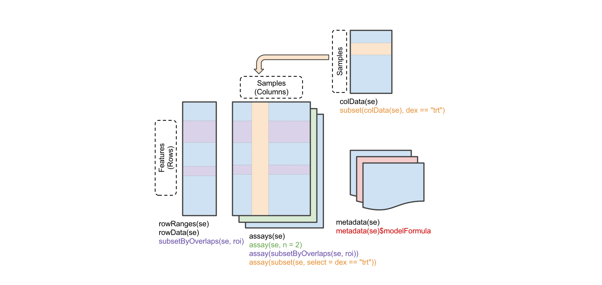
Alt SummarizedExperiment
Comprehensive data structure that can be used to store expression and methylation data from microarrays or read counts from RNA-seq experiments, among others.
Can contain slots for one or more omic datasets, feature annotation (e.g. genes, transcripts, SNPs, CpGs), individual phenotypes and experimental details, such as laboratory and experimental protocols.
As in an
ExpressionSetaSummarizedExperiment, the rows of omic data are features and columns are subjects.Coordinate feature x sample ‘assays’ with row (feature) and column (sample) descriptions.
‘assays’ (similar to ‘exprs’ in
ExpressionSetobjects) can be any matrix-like object, including very large on-disk representations such as HDF5Array‘assays’ are annotated using
GenomicRangesIt is being deprecated
3.5 Ranged Summarized Experiments
SummarizedExperiment is extended to RangedSummarizedExperiment, a child class that contains the annotation data of the features in a GenomicRanges object. An example dataset, stored as a RangedSummarizedExperiment is available in the airway package. This data represents an RNA sequencing experiment.
class: RangedSummarizedExperiment
dim: 64102 8
metadata(1): ''
assays(1): counts
rownames(64102): ENSG00000000003 ENSG00000000005 ... LRG_98 LRG_99
rowData names(0):
colnames(8): SRR1039508 SRR1039509 ... SRR1039520 SRR1039521
colData names(9): SampleName cell ... Sample BioSample- Some aspects of the object are very similar to
ExpressionSet, although with slightly different names and types.colDatacontains phenotype (sample) information, likepDataforExpressionSet. It returns aDataFrameinstead of a data.frame:
DataFrame with 8 rows and 9 columns
           SampleName     cell      dex    albut        Run avgLength Experiment    Sample    BioSample
             <factor> <factor> <factor> <factor>   <factor> <integer>   <factor>  <factor>     <factor>
SRR1039508 GSM1275862  N61311     untrt    untrt SRR1039508       126  SRX384345 SRS508568 SAMN02422669
SRR1039509 GSM1275863  N61311     trt      untrt SRR1039509       126  SRX384346 SRS508567 SAMN02422675
SRR1039512 GSM1275866  N052611    untrt    untrt SRR1039512       126  SRX384349 SRS508571 SAMN02422678
SRR1039513 GSM1275867  N052611    trt      untrt SRR1039513        87  SRX384350 SRS508572 SAMN02422670
SRR1039516 GSM1275870  N080611    untrt    untrt SRR1039516       120  SRX384353 SRS508575 SAMN02422682
SRR1039517 GSM1275871  N080611    trt      untrt SRR1039517       126  SRX384354 SRS508576 SAMN02422673
SRR1039520 GSM1275874  N061011    untrt    untrt SRR1039520       101  SRX384357 SRS508579 SAMN02422683
SRR1039521 GSM1275875 N061011 trt untrt SRR1039521 98 SRX384358 SRS508580 SAMN02422677- You can still use
$to get a particular column:
[1] N61311  N61311  N052611 N052611 N080611 N080611 N061011 N061011
Levels: N052611 N061011 N080611 N61311- The measurement data are accessed by
assayandassays. ASummarizedExperimentcan contain multiple measurement matrices (all of the same dimension). You get all of them by assays and you select a particular one byassay(OBJECT, NAME)where you can see the names when you print the object or by usingassayNames. In this case there is a single matrix called counts:
[1] "counts"List of length 1
names(1): counts SRR1039508 SRR1039509 SRR1039512 SRR1039513 SRR1039516 SRR1039517 SRR1039520 SRR1039521
ENSG00000000003 679 448 873 408 1138 1047 770 572
ENSG00000000005 0 0 0 0 0 0 0 0
ENSG00000000419 467 515 621 365 587 799 417 508
ENSG00000000457 260 211 263 164 245 331 233 229
ENSG00000000460 60 55 40 35 78 63 76 60
ENSG00000000938 0 0 2 0 1 0 0 0- Annotation is a
GenomicRangesobject
GRangesList object of length 64102:
$ENSG00000000003
GRanges object with 17 ranges and 2 metadata columns:
       seqnames            ranges strand |   exon_id       exon_name
          <Rle>         <IRanges>  <Rle> | <integer>     <character>
   [1]        X 99883667-99884983      - |    667145 ENSE00001459322
   [2]        X 99885756-99885863      - |    667146 ENSE00000868868
   [3]        X 99887482-99887565      - |    667147 ENSE00000401072
   [4]        X 99887538-99887565      - |    667148 ENSE00001849132
   [5]        X 99888402-99888536      - |    667149 ENSE00003554016
   ...      ...               ...    ... .       ...             ...
  [13]        X 99890555-99890743      - |    667156 ENSE00003512331
  [14]        X 99891188-99891686      - |    667158 ENSE00001886883
  [15]        X 99891605-99891803      - |    667159 ENSE00001855382
  [16]        X 99891790-99892101      - |    667160 ENSE00001863395
  [17]        X 99894942-99894988      - |    667161 ENSE00001828996
  -------
  seqinfo: 722 sequences (1 circular) from an unspecified genome

...
<64101 more elements>- Subset for only rows (e.g. features) which are in the interval 1 to 1Mb of chromosome 1
class: RangedSummarizedExperiment
dim: 79 8
metadata(1): ''
assays(1): counts
rownames(79): ENSG00000177757 ENSG00000185097 ... ENSG00000272512 ENSG00000273443
rowData names(0):
colnames(8): SRR1039508 SRR1039509 ... SRR1039520 SRR1039521
colData names(9): SampleName cell ... Sample BioSample
3.6 Multi Data Set
MultiDataSet is designed for integrating multi omic datasets.
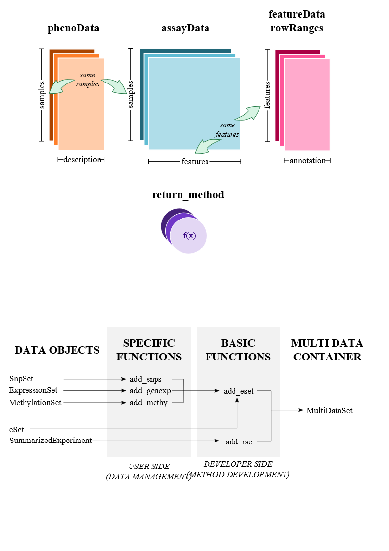
Alt MultiDataSet
Designed to encapsulate different types of datasets (including all classes in Bioconductor)
It properly deals with non-complete cases situations
Subsetting is easily performed in both: samples and features (using GenomicRanges)
It allows to: – perform integration analysis with third party packages; – create new methods and functions for omic data integration; – encapsule new unimplemented data from any biological experiment
MultiAssayExperiment is another infrastructure container (created by BioC developers) that can be used to manage multi-omic data