3 Epigenome-wide association study (EWAS)
In this chapter we will run an Epigenome-Wide Association Study (EWAS). A file with the slides can be downloaded here
At the end of the practice, please answer these questions:
- Which is the lambda of the unadjusted EWAS of current smoking? How does it change in adding covariates and surrogate variables?
- How many CpGs are associated with current smoking (after False Discovery Rate – FDR - correction) in the model adjusted by covariates and sva?
- How many of the FDR CpGs show higher methylation and how many lower methylation?
- Which is the top 1 CpG? In which chromosome is located?
3.2 Load dataset and extract the phenotypes and methylation matrix
We begin loading the output from the last step, which is the ExpressionSet that
contains the normalised betas together with the phenotype.
eset.cohort1<-readRDS("./data/DAY3/Input/GSE42861_norm_cohort1.Rds")

eset.cohort1
## ExpressionSet (storageMode: lockedEnvironment)
## assayData: 37842 features, 294 samples
## element names: exprs
## protocolData: none
## phenoData
## sampleNames: GSM1051533 GSM1051534 ... GSM1052213 (294 total)
## varLabels: Celltype Age ... NK (10 total)
## varMetadata: labelDescription
## featureData: none
## experimentData: use 'experimentData(object)'
## Annotation:Use pData() function from Biobase R package to extract cohort 1 phenodata
and exprs() function from Biobase R package to extract the cohort 1 methylation matrix.
## [1] 294 10
head(pheno.cohort1)## [1] 37842 294
methyl.cohort1[1:5,1:5]## GSM1051533 GSM1051534 GSM1051536 GSM1051537 GSM1051538
## cg02432075 0.09914671 0.05285574 0.11479000 0.09238820 0.05655322
## cg03515901 0.90775178 0.91091962 0.91043927 0.89217759 0.91384704
## cg04023335 0.64876572 0.53111687 0.57309345 0.37877619 0.59618924
## cg08455548 0.07235159 0.07022040 0.09489939 0.08827584 0.06616870
## cg00006815 0.04753770 0.05215979 0.04847625 0.06924370 0.039708453.3 Run EWAS
3.3.1 Data preparation
Here we will show an example to run the analysis testing never smokers against current smokers. Nevertheless, the same code can be applied to run other analyses testing never vs former.
The first step is to subset the ExpressionSet with only the samples that we need.
In this case, we only keep the never smokers and the current smokers,
getting rid of the former smokers.
table(pheno.cohort1$Smoking)##
## current former never
## 89 106 99## [1] 188 10
eset.current <- eset.cohort1[,rownames(current)] #subset the eset
eset.current
## ExpressionSet (storageMode: lockedEnvironment)
## assayData: 37842 features, 188 samples
## element names: exprs
## protocolData: none
## phenoData
## sampleNames: GSM1051533 GSM1051534 ... GSM1052213 (188 total)
## varLabels: Celltype Age ... NK (10 total)
## varMetadata: labelDescription
## featureData: none
## experimentData: use 'experimentData(object)'
## Annotation:
table(eset.current$Smoking)##
## current never
## 89 99Extract phenodata from the ExpressionSet with never and current smokers
using pData() function from Biobase R package.
Now, we need to check the exposure variable (Smoking). We need this variable as factor.
## [1] "factor"Check the levels. We want “never” to be the reference level.To this end, you
can use the relevel()function.
levels(pheno.current$Smoking)## [1] "current" "never"## [1] "never" "current"Finally, create an object with the exposure variable (Smoking).
You will need this object to run the meffil.ewas() function.
variable <- pheno.current$Smoking
class(variable)
## [1] "factor"The next step is to select the covariates of interest for the EWAS. We are interested in sex, age and cell type proportions. Check the class of these covariates before running the analysis.
class(pheno.current$Age)## [1] "integer"
class(pheno.current$Sex)## [1] "character"
class(pheno.current$Bcell)## [1] "numeric"
class(pheno.current$CD4T)## [1] "numeric"
class(pheno.current$CD8T)## [1] "numeric"
class(pheno.current$Mono)## [1] "numeric"
class(pheno.current$Neu)## [1] "numeric"
class(pheno.current$NK)## [1] "numeric"Then, create a new data.framewith the covariates of interest.
You will need this object to run the meffil.ewas() function.
pheno.current$Sex<-as.factor(pheno.current$Sex)
covariates <- pheno.current[,c("Age","Sex",
                               "Bcell","CD4T","CD8T","Mono","Neu","NK")]
After having the exposure and the covariates objects ready, you will need to
extract the methylation matrix from the ExpressionSet using exprs() function
from Biobase R package. You will need this object to run the meffil.ewas() function.
methyl.current<-exprs(eset.current)
methyl.current[1:5,1:5]
## GSM1051533 GSM1051534 GSM1051539 GSM1051541 GSM1051542
## cg02432075 0.09914671 0.05285574 0.08496137 0.09643806 0.09607922
## cg03515901 0.90775178 0.91091962 0.92017725 0.88514304 0.93523586
## cg04023335 0.64876572 0.53111687 0.57413506 0.52785496 0.64774883
## cg08455548 0.07235159 0.07022040 0.08805554 0.08864486 0.11191411
## cg00006815 0.04753770 0.05215979 0.05949175 0.05490687 0.05724176Check order of the samples between the pheno and the methylation matrix. If samples are not in the same order, you could incorrectly assign the values of the variables to the samples and therefore also to the methylation.
##
## Matched
##     188
3.3.2 EWAS
To run the EWAS we will use the function meffil.ewas() from meffil R package.
We need as arguments:
- beta: Methylation matrix
- variable: Vector with the exposure variable.
- covariates: A dataframe with the covariates to include in the regression model
- rlm: As we want to run a robust linear regression model, we need to specify “TRUE” in the argument “rlm”
- winsorize.pct: To reduce the impact of severe outliers in the DNA methylation data, we will winsorize the methylation beta values (1%), with 0.5% at upper and lower ends of the distribution (Ghosh 2012)
- sva (by default TRUE). This function will apply Surrogate Variable Analysis (SVA) to the methylation levels and covariates and include the resulting variables as covariates in the regression model to correct for technical batch (noise)
ewas.current <- meffil.ewas(methyl.current,
                            variable=variable,
                            covariates=covariates,
                            rlm=TRUE,
                            winsorize.pct=0.05)
## Number of significant surrogate variables is: 31
## Iteration (out of 5 ):1 2 3 4 53.3.3 Results
We obtain an object with several information
summary(ewas.current)## Length Class Mode
## class 1 -none- character
## version 1 package_version list
## samples 188 -none- character
## variable 188 factor numeric
## covariates 8 data.frame list
## winsorize.pct 1 -none- numeric
## batch 0 -none- NULL
## robust 1 -none- logical
## rlm 1 -none- logical
## weights 0 -none- NULL
## outlier.iqr.factor 1 -none- logical
## most.variable 1 -none- numeric
## p.value 113526 -none- numeric
## coefficient 113526 -none- numeric
## analyses 3 -none- list
## random.seed 1 -none- numeric
## sva.ret 4 -none- listWe are interested in the EWAS results. This function calculated the results
1) without adjusting for covariates, 2) adjusting for the covariates we specified above
and also 3) adjusting for the covariates and the surrogate variables to correct the batch (noise)
summary(ewas.current$analyses)## Length Class Mode
## none 5 -none- list
## all 5 -none- list
## sva 5 -none- listWe will use the results from the analysis adjusted for the covariates and the surrogate variables
res.current<-ewas.current$analyses$sva
res.current<-res.current$table
We will create a column with the Probe ID, which now is in the rows of the results dataframe
res.current$probeID<-rownames(res.current)We order the results by p.value
The column names stand for:
- p.value: pval significance of the association
- fdr: p.value corrected by the FALSE DISCOVERY RATE method
- p.holm: p.value corrected by Holm-Bonferroni method (we are not going to use it)
- t.statistic
- coefficient: coefficient of the association (the effect or beta)
- coefficient.ci.high: confidence interval up
- coefficient.ci.low: confindence interval down
- coefficient.se: standard error of the coefficient
- n: sample size included in the analysis
- chromosome: chromosome in which the CpG is located in the genome (hg19)
- position: position of the CpG in the genome (hg19)
Significant hits
Our results were corrected for multiple testing using FDR method. Significance was defined at FDR p-value < 0.05. We tested 37,842 CpGs.
dim(res.current.ord)## [1] 37842 12Significant CpGs with a FDR p-value <0.05
res.current.sig<-res.current.ord[res.current.ord$fdr < 0.05,]
dim(res.current.sig)
## [1] 289 12
head(res.current.sig)Number of significant CpGs with a positive or negative effect
dim(res.current.sig[res.current.sig$coefficient <0,]) ## [1] 164 12
dim(res.current.sig[res.current.sig$coefficient >0,]) ## [1] 125 123.3.4 Report
To explore the results, we will create a report using meffil.ewas.parameters() and meffil.ewas.summary() functions from meffil R package.
This report contains:
- Sample characteristics
- Covariate associations: Associations between the exposure variable (Smoking) and the covariates.
- Lambdas and QQplots to examine inflation (none, all cov, sva)
- Manhattan plots
- Significant CpG sites. As threshold we will indicate FDR=0.05.
- Specific CpGs Box plot: To observe the methylation differences between Never VS Current smokers, you can specify the CpGs that you are interested in. Today we will select our top significant CpG “cg05575921” that is annotated to AHRR gene and it is well known for its association with tabbacco.
ewas.parameters <- meffil.ewas.parameters(max.plots = 1,model="sva", sig.threshold = 3.86e-04) #FDR (0.05) = p.value (3.86e-04)
candidate.site <- c("cg05575921")
ewas.summary <- meffil.ewas.summary(ewas.current,
                                    methyl.current,
                                    selected.cpg.sites=candidate.site,
                                    parameters=ewas.parameters)
DO NOT RUN THIS STEP IN THE VIRTUAL MACHINE - The report can be found here
meffil.ewas.report(ewas.summary,
                   output.file="./data/DAY3/Output/Report.EWAS.cohort1.NeverVScurrent_student.html")
## [meffil.ewas.report] Wed Sep 6 00:09:30 2023 Writing report as html file to ./data/DAY3/Output/Report.EWAS.cohort1.NeverVScurrent_student.html3.3.5 Plots
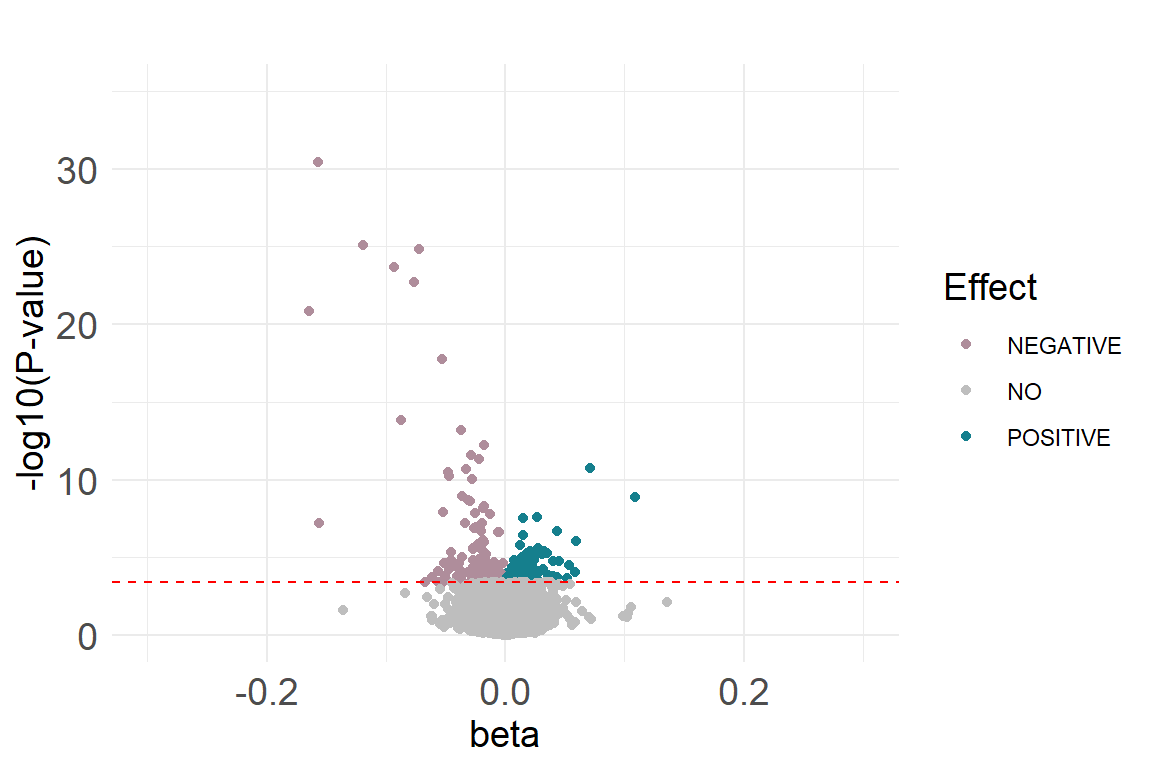
Volcano plot
The plot that you should obtain can be found here
res.current.ord$diffexpressed <- "NO"
res.current.ord$diffexpressed[res.current.ord$coefficient > 0
                              & res.current.ord$fdr <0.05] <- "POSITIVE"
res.current.ord$diffexpressed[res.current.ord$coefficient < 0
                              & res.current.ord$fdr <0.05] <- "NEGATIVE"

p <- ggplot(data=res.current.ord, aes(x=res.current.ord$coefficient, y=-log10(res.current.ord$p.value), col=res.current.ord$diffexpressed)) +
  xlim(c(-0.3,0.3))+ ylim(c(0,35)) +
  geom_point(size = 1.5) + theme_minimal() +
  labs(title = " ", x = "beta", y = "-log10(P-value)", colour = "Effect") +
  theme(axis.title = element_text(size = 14, color = "black",vjust=0.5)) +
  theme(plot.title = element_text(size = 14,face="bold",color="black",
                                  hjust= 0.5, vjust=0.5)) +
  theme(legend.title = element_text(color = "black", size = 14))


# Add lines as before...
p2 <- p + geom_hline(yintercept=c(-log10(3.86e-04)), col=c("red"),
                     linetype = "dashed") +
  theme(axis.text = element_text(size = 14)) #thres FDR (0.05) = p.val 3.86-04
mycolors<-c("#157F8D","#AF8D9B", "grey")
names(mycolors) <- c("POSITIVE", "NEGATIVE", "NO")

p3 <- p2 + scale_colour_manual(values = mycolors)

p3
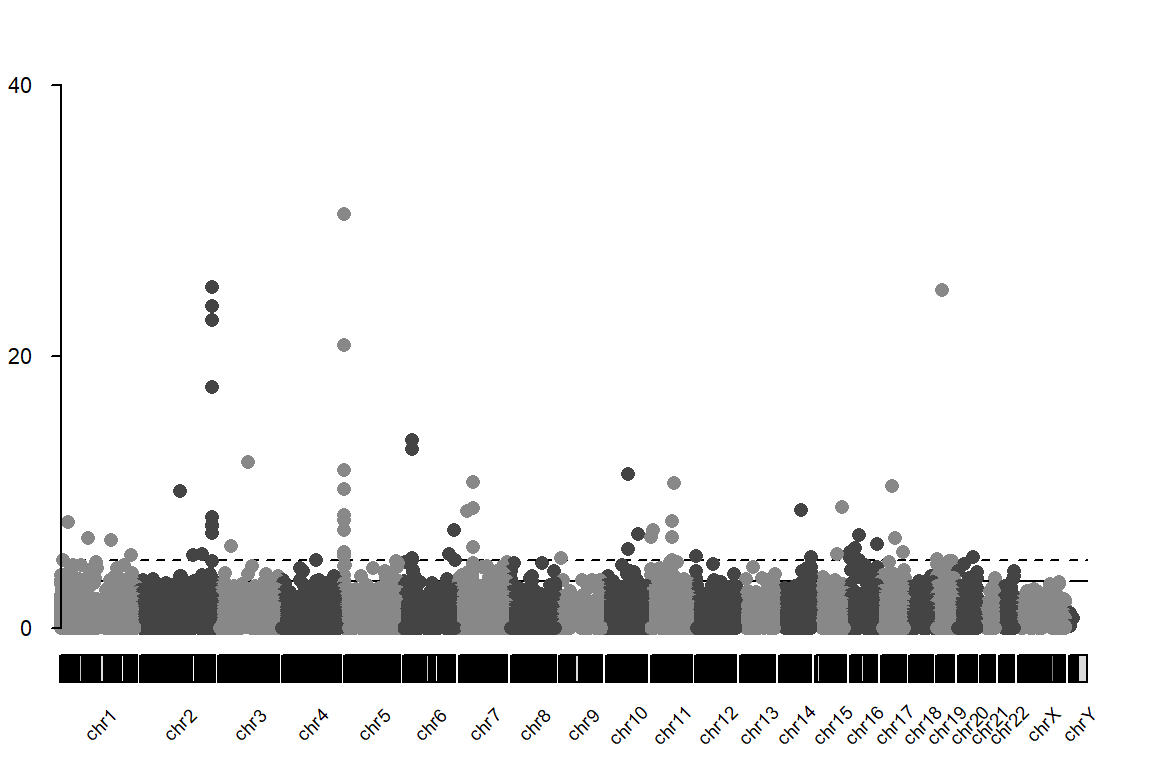
Manhattan plot
The plot that you should obtain can be found here
# Create a dataframe with chr, start, end and pval
df.current<-res.current.ord[,c("chromosome","position","p.value")]
head(df.current)
df.current$start<-df.current$position
df.current$end<-df.current$position + 1
colnames(df.current)<-c("chr","position","p.value","start","end")
df.current<-df.current[,c("chr","start","end","p.value")]

# Create GRanges object needed
df.GRanges<-makeGRangesFromDataFrame(df.current, keep.extra.columns = TRUE)

kp <- plotKaryotype(plot.type=4, labels.plotter = NULL)
kp <- kpAddChromosomeNames(kp, cex=0.6, srt=45)
kp <- kpPlotManhattan(kp, data=df.GRanges,pval=df.current$p.value, ymax=40,genomewideline =3.42)
kp <- kpAxis(kp, ymin=0, ymax=40, cex=0.7)
ANSWERS
- Unadjusted: 2.44, adjusted for covariates: 2.22 and adjusted for covariates + sva: 1.51
- 289
- 164 show a negative effect and 125 show a positive effect
- cg05575921, it is located in chromosome 5
