4 Genome-wide association studies
In this chapter we explain how to perform genome-wide association studies (GWAS), where high-dimensional genomic data is treated. Issues concerning quality control of SNPs and individuals are discussed, as well as association tests and possible sources of confounding such as population stratification. We finish SNP analyses with tools that help to interpret results (e.g. post-omic data analyses).
GWAS assess the association between the trait of interest and up to millions of SNPs. GWAS have been used to discover thousands of SNPsassociated with several complex diseases (MacArthur et al. 2016). The basic statistical methods are similar to those previously described, in particular, the massive univariate testing. The main issue with GWAS is data management and computation. Most publicly available data is in PLINK format, where genomic data is stored in a binary BED file, and phenotype and annotation data in text BIM and FAM files. PLINK data can be loaded into R with the Bioconductor’s package snpStats.
We illustrate the analysis of a GWAS including 100,000 SNPs that have been simulated using real data from a case-control study. Our phenotype of interest is obesity (0: not obese; 1: obese) that has been created using body mass index information of each individual. We start by loading genotype data that are in PLINK format (obesity.bed, obesity.bim, obesity.fam files).
library(snpStats)
path <- "data"
ob.plink <- read.plink(file.path(path, "obesity"))
The imported object is a list containing the genotypes, the family structure and the SNP annotation.
names(ob.plink)[1] "genotypes" "fam" "map" We store genotype, annotation and family data in different variables for downstream analyses
ob.geno <- ob.plink$genotypes
ob.geno
A SnpMatrix with 2312 rows and 100000 columns
Row names: 100 ... 998
Col names: MitoC3993T ... rs28600179 annotation <- ob.plink$map
head(annotation) chromosome snp.name cM position allele.1 allele.2
MitoC3993T NA MitoC3993T NA 3993 T C
MitoG4821A NA MitoG4821A NA 4821 A G
MitoG6027A NA MitoG6027A NA 6027 A G
MitoT6153C NA MitoT6153C NA 6153 C T
MitoC7275T NA MitoC7275T NA 7275 T C
MitoT9699C NA MitoT9699C NA 9699 C Tfamily <- ob.plink$fam
head(family) pedigree member father mother sex affected
100 FAM_OB 100 NA NA 1 1
1001 FAM_OB 1001 NA NA 1 1
1004 FAM_OB 1004 NA NA 2 2
1005 FAM_OB 1005 NA NA 1 2
1006 FAM_OB 1006 NA NA 2 1
1008 FAM_OB 1008 NA NA 1 1Notice that geno is an object of class SnpMatrixthat stores the SNPs in binary (raw) format. While some basic phenotype data is usually available in the fam field of the SnpMatrix object, a more complete phenotypic characterization of the sample is usually distributed in additional text files. In our example, the complete phenotype data is in a tab-delimited file
ob.pheno <- read.delim(file.path(path, "obesity.txt"))
head(ob.pheno)
scanID gender obese age smoke country asthma
1 100 Male 0 48 Never 53 1
2 1001 Male 1 49 Never 54 1
3 1004 Female 0 38 Ex 51 2
4 1005 Male 0 39 Never 53 2
5 1006 Female 0 43 Ex 53 1
6 1008 Male 1 49 Never 55 1The file contains phenotypic information for a different set of individuals that overlap with those in the ob.geno object. Therefore, before analysis, we need to correctly merge and order the individuals across genomic and phenotype datasets. The row names of ob.geno correspond to the individual identifiers (id) variable of ob.pheno. Consequently, we also rename the rows of ob.pheno with the id variable
rownames(ob.pheno) <- ob.pheno$scanIDWe can check if the row names of the datasets match
identical(rownames(ob.pheno), rownames(ob.geno))[1] TRUEFALSE indicates that either there are different individuals in both objects or that they are in different order. This can be fixed by selecting common individuals.
ids <- intersect(rownames(ob.pheno), rownames(ob.geno))
geno <- ob.geno[ids, ]
ob <- ob.pheno[ids, ]
identical(rownames(ob), rownames(geno))
[1] TRUEfamily <- family[ids, ]4.1 Quality control of SNPs
We now perform the quality control (QC)of genomic data at the SNP and individual levels, before association testing (Anderson et al. 2010). Different measures can be used to perform QC and remove:
- SNPs with a high rate of missing;
- rare SNPS (e.g. having low minor allele frequency (MAF); and
- SNPs that do not pass the HWE test.
Typically, markers with a call rate less than 95% are removed from association analyses, although some large studies chose higher call-rate thresholds (99%). Markers of low MAF (\(<5\)%) are also filtered. The significance threshold rejecting a SNP for not being in HWE has varied greatly between studies, from thresholds between 0.001 and \(5.7 \times 10^{-7}\) (Clayton et al. 2005). Including SNPs with extremely low \(P\)-values for the HWE test will require individual examination of the SNP genotyping process. A parsimonious threshold of 0.001 may be considered, though robustly genotyped SNPs below this threshold may remain in the study (Anderson et al. 2010), as deviations from HWE may indeed arise from biological processes.
The function col.summary() offers different summaries (at SNP level) that can be used in QC
info.snps <- col.summary(geno)
head(info.snps)
Calls Call.rate Certain.calls RAF MAF
MitoC3993T 2286 0.9887543 1 0.9851269 0.0148731409
MitoG4821A 2282 0.9870242 1 0.9982472 0.0017528484
MitoG6027A 2307 0.9978374 1 0.9956654 0.0043346337
MitoT6153C 2308 0.9982699 1 0.9893847 0.0106152513
MitoC7275T 2309 0.9987024 1 0.9991338 0.0008661758
MitoT9699C 2302 0.9956747 1 0.9268028 0.0731972198
P.AA P.AB P.BB z.HWE
MitoC3993T 0.0148731409 0.0000000000 0.9851269 -47.81213
MitoG4821A 0.0017528484 0.0000000000 0.9982472 -47.77028
MitoG6027A 0.0043346337 0.0000000000 0.9956654 -48.03124
MitoT6153C 0.0103986135 0.0004332756 0.9891681 -47.05069
MitoC7275T 0.0008661758 0.0000000000 0.9991338 -48.05206
MitoT9699C 0.0729800174 0.0004344049 0.9265856 -47.82555snpStats does not compute \(P\)-values of the HWE test but computes its \(z\)-scores. A \(P\)-value of 0.001 corresponds to a \(z\)-score of \(\pm 3.3\) for a two-tail test. Strictly speaking, the HWE test should be applied to controls only (e.g. obese = 0). However, the default computation is for all samples.
We thus filter SNPs with a call rate \(>95\%\), MAF of \(>5\%\) and \(z.HWE<3.3\) in controls
controls <- ob$obese ==0 & !is.na(ob$obese)
geno.controls <- geno[controls,]
info.controls <- col.summary(geno.controls)

use <- info.snps$Call.rate > 0.95 &
       info.snps$MAF > 0.05 &
       abs(info.controls$z.HWE < 3.3)
mask.snps <- use & !is.na(use)

geno.qc.snps <- geno[ , mask.snps]
geno.qc.snps
A SnpMatrix with 2312 rows and 88723 columns
Row names: 100 ... 998
Col names: MitoT9699C ... rs28562204 annotation <- annotation[mask.snps, ]It is common practice to report the number of SNPs that have been removed from the association analyses
# number of SNPs removed for bad call rate
sum(info.snps$Call.rate < 0.95)
[1] 888# number of SNPs removed for low MAF
sum(info.snps$MAF < 0.05, na.rm=TRUE)[1] 10461#number of SNPs that do not pass HWE test
sum(abs(info.controls$z.HWE > 3.3), na.rm=TRUE) [1] 80# The total number of SNPs do not pass QC
sum(!mask.snps)[1] 112774.2 Quality control of individuals
QC of individuals, or biological samples, comprises four main steps (Anderson et al. 2010):
- The identification of individuals with discordant reported and genomic sex,
- the identification of individuals with outlying missing genotype or heterozygosity rate,
- the identification of duplicated or related individuals, and
- the identification of individuals of divergent ancestry from the sample.
We start by removing individuals with sex discrepancies, a large number of missing genotypes and outlying heterozygosity. The function row.summary() returns the call rate and the proportion of called SNPs which are heterozygous per individual.
info.indv <- row.summary(geno.qc.snps)
head(info.indv)
Call.rate Certain.calls Heterozygosity
100 0.9991547 1 0.3399851
1001 0.9987151 1 0.3456195
1004 0.9953451 1 0.3499943
1005 0.9996168 1 0.3415643
1006 0.9990983 1 0.3482170
1008 0.9995041 1 0.3435763Gender is usually inferred from the heterozygosity of chromosome X. Males have an expected heterozygosity of 0 and females of 0.30. Chromosome X heterozygosity can be extracted using row.summary() function and then plotted
geno.X <- geno.qc.snps[,annotation$chromosome=="23" &
                         !is.na(annotation$chromosome)]
info.X <- row.summary(geno.X)
mycol <- ifelse(ob$gender=="Male", "gray40", "gray80")
plot(info.X$Heterozygosity, col=mycol,
     pch=16, xlab="Individuals",
     ylab="Heterozygosity in chromosome X")
legend("topright", c("Males", "Females"), col=mycol,
       pch=16)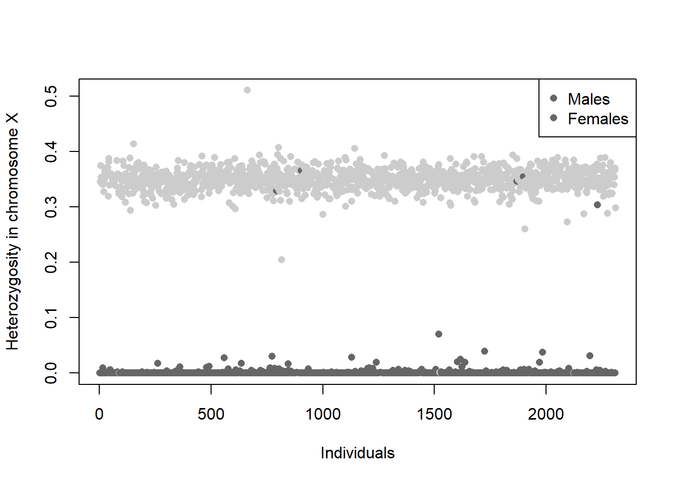
Figure 4.1: Heterozygosity in chromosome X by gender provided in the phenotypic data.
Figure 4.1 shows that there are some reported males with non-zero X-heterozygosity and females with zero X-heterozygosity. These samples are located in sex.discrep for later removal
sex.discrep <- (ob$gender=="Male" & info.X$Heterozygosity > 0.2) |
               (ob$gender=="Female" & info.X$Heterozygosity < 0.2)
Sex filtering based on X-heterozygosity is not sufficient to identify rare aneuploidies, like XXY in males. Alternatively, plots of the mean allelic intensities of SNPs on the X and Y chromosomes can identify mis-annotated sex as well as sex chromosome aneuploidies.
Now, we identify individuals with outlying heterozygosity from the overall genomic heterozygosity rate that is computed by the function row.summary(). Heterozygosity, can also be computed from the statistic \(F = 1 - \frac{f(Aa)}{E(f(Aa))}\), where \(f(Aa)\) is the observed proportion of heterozygous genotypes (Aa) of a given individual and \(E(f(Aa))\) is the expected proportion of heterozygous genotypes. A subject’s \(E(f(Aa))\) can be computed from the MAF across all the subjects’ non-missing SNPs
MAF <- col.summary(geno.qc.snps)$MAF
callmatrix <- !is.na(geno.qc.snps)
hetExp <- callmatrix %*% (2*MAF*(1-MAF))
hetObs <- with(info.indv, Heterozygosity*(ncol(geno.qc.snps))*Call.rate)
info.indv$hetF <- 1-(hetObs/hetExp)

head(info.indv)
Call.rate Certain.calls Heterozygosity hetF
100 0.9991547 1 0.3399851 0.031007624
1001 0.9987151 1 0.3456195 0.014898707
1004 0.9953451 1 0.3499943 0.002145765
1005 0.9996168 1 0.3415643 0.026466552
1006 0.9990983 1 0.3482170 0.007425401
1008 0.9995041 1 0.3435763 0.020744532In Figure 4.2, we compare \(F\) statistic and the Heterozygosity obtained from row.summary()
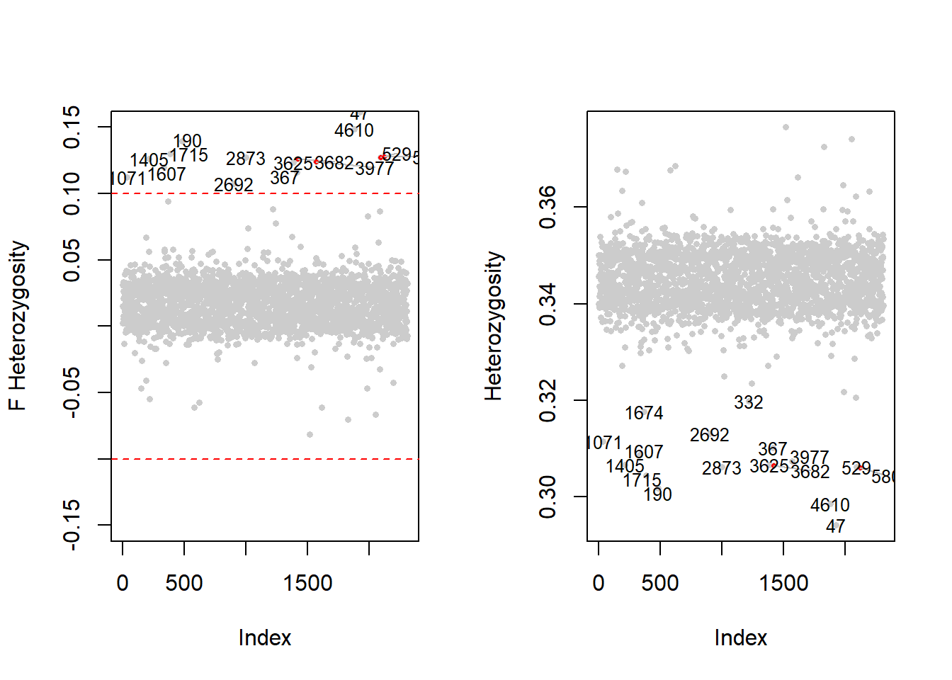
Figure 4.2: Heterozygosity computed using F statistic (left panel) and using row.summary function (right panel). The horizontal dashed line shows a suggestive value to detect individuals with outlier heterozygosity values.
Individuals whose \(F\) statistic is outside the band \(\pm 0.1\) are considered sample outliers (left panel Figure 4.2 and correspond to those having a heterozygosity rate lower than 0.32.
GWASs are studies that are typically based on population samples. Therefore, close familial relatedness between individuals is not representative of the sample. We, therefore, remove individuals whose relatedness is higher than expected. The package SNPRelate is used to perform identity-by-descent (IBD) analysis, computing kinship within the sample. The package requires a data in a GDS format that is obtained with the function snpgdsBED2GDS. In addition, IBD analysis requires SNPs that are not in LD (uncorrelated). The function snpgdsLDpruning iteratively removes adjacent SNPs that exceed an LD threshold in a sliding window
library(SNPRelate)

# Transform PLINK data into GDS format
snpgdsBED2GDS("data/obesity.bed",
              "data/obesity.fam",
              "data/obesity.bim",
              out="obGDS")
Start file conversion from PLINK BED to SNP GDS ...
BED file: "data/obesity.bed"
SNP-major mode (Sample X SNP), 55.1M
FAM file: "data/obesity.fam"
BIM file: "data/obesity.bim"
Wed Nov 11 09:32:28 2020 (store sample id, snp id, position, and chromosome)
start writing: 2312 samples, 100000 SNPs ...
[..................................................] 0%, ETC: ---
[==================================================] 100%, completed, 1s
Wed Nov 11 09:32:29 2020 Done.
Optimize the access efficiency ...
Clean up the fragments of GDS file:
open the file 'obGDS' (55.7M)
# of fragments: 39
save to 'obGDS.tmp'
rename 'obGDS.tmp' (55.7M, reduced: 252B)
# of fragments: 18genofile <- snpgdsOpen("obGDS")
# Prune SNPs for IBD analysis
set.seed(12345)
snps.qc <- colnames(geno.qc.snps)
snp.prune <- snpgdsLDpruning(genofile, ld.threshold = 0.2,
snp.id = snps.qc)SNP pruning based on LD:
Excluding 13,410 SNPs (non-autosomes or non-selection)
Excluding 0 SNP (monomorphic: TRUE, MAF: NaN, missing rate: NaN)
# of samples: 2,312
# of SNPs: 86,590
using 1 thread
sliding window: 500,000 basepairs, Inf SNPs
|LD| threshold: 0.2
method: composite
Chromosome 1: 31.58%, 2,438/7,721
Chromosome 2: 29.98%, 2,413/8,050
Chromosome 3: 30.83%, 2,058/6,676
Chromosome 4: 30.94%, 1,834/5,927
Chromosome 5: 31.05%, 1,886/6,074
Chromosome 6: 28.18%, 1,902/6,750
Chromosome 7: 31.27%, 1,675/5,356
Chromosome 8: 28.86%, 1,608/5,572
Chromosome 9: 31.62%, 1,492/4,718
Chromosome 10: 30.73%, 1,595/5,191
Chromosome 11: 30.93%, 1,476/4,772
Chromosome 12: 31.64%, 1,536/4,855
Chromosome 13: 31.36%, 1,142/3,642
Chromosome 14: 32.72%, 1,063/3,249
Chromosome 15: 31.76%, 972/3,060
Chromosome 16: 35.62%, 1,059/2,973
Chromosome 17: 36.24%, 986/2,721
Chromosome 18: 34.11%, 1,005/2,946
Chromosome 19: 40.80%, 694/1,701
Chromosome 20: 35.66%, 859/2,409
Chromosome 21: 34.83%, 488/1,401
Chromosome 22: 34.61%, 552/1,595
30,733 markers are selected in total.snps.ibd <- unlist(snp.prune, use.names=FALSE)Note that this process is performed with SNPs that passed previous QC checks. IBD coefficients are then computed using the method of moments, implemented in the function snpgdsIBDMoM(). The result of the analysis is a table indicating kinship among pairs of individuals
ibd <- snpgdsIBDMoM(genofile, kinship=TRUE,
                    snp.id = snps.ibd,
                    num.thread = 1)
IBD analysis (PLINK method of moment) on genotypes:
Excluding 69,267 SNPs (non-autosomes or non-selection)
Excluding 0 SNP (monomorphic: TRUE, MAF: NaN, missing rate: NaN)
# of samples: 2,312
# of SNPs: 30,733
using 1 thread
PLINK IBD: the sum of all selected genotypes (0,1,2) = 32774873
Wed Nov 11 09:32:32 2020 (internal increment: 13952)
[..................................................] 0%, ETC: ---
[==================================================] 100%, completed, 9s
Wed Nov 11 09:32:41 2020 Done.ibd.kin <- snpgdsIBDSelection(ibd)
head(ibd.kin) ID1 ID2 k0 k1 kinship
1 100 1001 1 0 0
2 100 1004 1 0 0
3 100 1005 1 0 0
4 100 1006 1 0 0
5 100 1008 1 0 0
6 100 1013 1 0 0A pair of individuals with higher than expected relatedness are considered with kinship score \(> 0.1\)
ibd.kin.thres <- subset(ibd.kin, kinship > 0.1)
head(ibd.kin.thres)
ID1 ID2 k0 k1 kinship
46484 1049 188 0.2759234 0.5337773 0.2285940
232848 1202 1330 0.0000000 0.0000000 0.5000000
281069 1237 872 0.2874340 0.4451656 0.2449916
640474 155 1682 0.2377813 0.4570711 0.2668416
806337 170 2015 0.2564809 0.5414546 0.2363959
1158509 2055 825 0.0000000 0.0000000 0.5000000The ids of the individuals with unusual kinship are located with related() function from the SNPassoc package
ids.rel <-  SNPassoc::related(ibd.kin.thres)
ids.rel
[1] "4364" "3380" "2999" "2697" "2611" "2088" "1202" "872" "825"
[10] "684" "188" "170" "155" "2071"Summing up, individuals with more than 5% missing genotypes Silverberg et al. (2009), with sex discrepancies, \(F\) absolute value \(>1\) and kinship coefficient \(>0.1\) are removed from the genotype and phenotype data
use <- info.indv$Call.rate > 0.95 &
       abs(info.indv$hetF) < 0.1 &
       !sex.discrep &
       !rownames(info.indv)%in%ids.rel
mask.indiv <- use & !is.na(use)
geno.qc <- geno.qc.snps[mask.indiv, ]

ob.qc <- ob.pheno[mask.indiv, ]
identical(rownames(ob.qc), rownames(geno.qc))
[1] TRUEThese QC measures are usually reported
# number of individuals removed to bad call rate
sum(info.indv$Call.rate < 0.95)
[1] 34# number of individuals removed for heterozygosity problems
sum(abs(info.indv$hetF) > 0.1)[1] 15# number of individuals removed for sex discrepancies
sum(sex.discrep)[1] 8# number of individuals removed to be related with others
length(ids.rel)[1] 14# The total number of individuals that do not pass QC
sum(!mask.indiv)[1] 704.3 Population ancestry
As GWAS are based on general population samples, individual genetic differences between individuals need to be also representative of the population at large. The main source of genetic differences between individuals is ancestry. Therefore, it is important to check that there are not individuals with unexpected genetic differences in the sample. Ancestral differences can be inferred with principal component analysis (PCA) on the genomic data. Individuals with outlying ancestry can be removed from the study while smaller differences in ancestry can be adjusted in the association models, including the first principal components as covariates.
PCA on genomic data can be computed using the SNPRelate package with the snpgdsPCA() function. Efficiency can be improved by removing SNPs that are in LD before PCA, see snps.ibd object in the previous IBD analysis. In addition the functio snpgdsPCA() allows parallelization with the argument num.thread that determines the number of computing cores to be used
pca <- snpgdsPCA(genofile, sample.id = rownames(geno.qc),
                           snp.id = snps.ibd,
                           num.thread=1)
Principal Component Analysis (PCA) on genotypes:
Excluding 69,267 SNPs (non-autosomes or non-selection)
Excluding 0 SNP (monomorphic: TRUE, MAF: NaN, missing rate: NaN)
# of samples: 2,242
# of SNPs: 30,733
using 1 thread
# of principal components: 32
PCA: the sum of all selected genotypes (0,1,2) = 31788248
CPU capabilities: Double-Precision SSE2
Wed Nov 11 09:33:16 2020 (internal increment: 448)
[..................................................] 0%, ETC: ---
[==================================================] 100%, completed, 31s
Wed Nov 11 09:33:47 2020 Begin (eigenvalues and eigenvectors)
Wed Nov 11 09:33:52 2020 Done.A PCA plot for the first two components can be obtained with
with(pca, plot(eigenvect[,1], eigenvect[,2],
               xlab="1st Principal Component",
               ylab="2nd Principal Component",
               main = "Ancestry Plot",
               pch=21, bg="gray90", cex=0.8))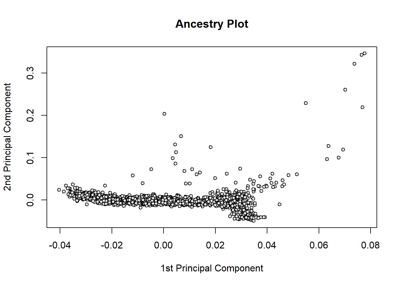
(#fig:pca_plot)1st and 2nd principal components of obesity GWAS data example.
Inspection of Figure @ref(fig:pca_plot) can be used to identify individuals with unusual ancestry and remove them. Individuals with outlying values in the principal components will be considered for QC. In our example, we can see outlying individuals on the right side of the plot with 1st PC \(> 0.05\). Smaller differences in ancestry are an important source of bias in association tests, as explained later. Therefore, we keep the first five principal components and add it to the phenotypic information that will be used in the association analyses.
ob.qc <- data.frame(ob.qc, pca$eigenvect[, 1:5])After performing QC, the GDS file can be closed
closefn.gds(genofile)4.4 Genome-wide association analysis
Genome-wide association analysis involves regressing each SNP separately on our trait of interest. The analyses should be adjusted for clinical, environmental, and/or demographic factors as well as ancestral differences between the subjects. The analysis can be performed with a range of functions in snpStats package. We first examine the unadjusted whole genome association of our obesity study
res <- single.snp.tests(obese, data=ob.qc,
                        snp.data=geno.qc)
res[1:5,]
N Chi.squared.1.df Chi.squared.2.df P.1df
MitoT9699C 2134 3.0263311 NA 0.08192307
MitoA11252G 2090 0.3561812 NA 0.55063478
MitoA12309G 2136 0.1776464 NA 0.67340371
MitoG16130A 2069 2.4766387 3.9480296 0.11554896
rs28705211 2125 0.7277258 0.7546827 0.39362135
P.2df
MitoT9699C NA
MitoA11252G NA
MitoA12309G NA
MitoG16130A 0.1388981
rs28705211 0.6856820This analysis is only available for the additive (\(\chi^2\)(1.df)) and the codominant models (\(\chi^2\)(2.df)). It requires the name variable phenotype (obese) in the data argument. Genomic data are given in the snp.data argument. It is important that the individuals in the rows of both datasets match. SNPs in the mitochondrial genome and gonosomes return NA for the \(\chi^2\) estimates. These variants should be analyzed separately. A common interest is to analyze autosomes only, and therefore these SNPs can be removed in the QC process.
A quantitative trait can also be analyzed setting the argument family equal to “Gaussian”
res.quant <- snp.rhs.tests(age ~ 1,  data=ob.qc,
                           snp.data=geno.qc,
                           family="Gaussian")
head(res.quant)
Chi.squared Df p.value
MitoT9699C 0.003422591 1 0.953348Population stratificationinflates the estimates of the \(\chi^2\) tests of association between the phenotype and the SNPs, and as a consequence the false positive rate increases. Figure @ref{fig:stratificationExample} illustrates why population stratification may lead to false associations. In the hypothetical study in the figure, we compare 20 cases and 20 controls where individuals carrying a susceptibility allele are denoted by a dot. The overall frequency of the susceptibility allele is much larger in cases (0.55 = 11/20) than in controls (0.35 = 7/20), the odds of being a case in allele carriers is $$2.3 times higher than the odds of being a case in non carriers (OR= 2.27 = (0.55/0.45) / (0.35/0.65)). However, the significant increase in susceptibility between the allele is misleading, as the OR in population A (light color) is 0.89 and in population B (dark color) is 1.08. The susceptibility allele strongly discriminates population A from B, and given the differences of the trait frequency between populations, it is likely that the association of the allele with the trait is through its links with population differences and not with the trait itself.
In genome-wide analyses, the inflation of the associations due to undetected latent variables is assessed by quantile-quantile (Q-Q) plots where observed \(\chi^2\) values are plotted against the expected ones
chi2 <- chi.squared(res, df=1)
qq.chisq(chi2)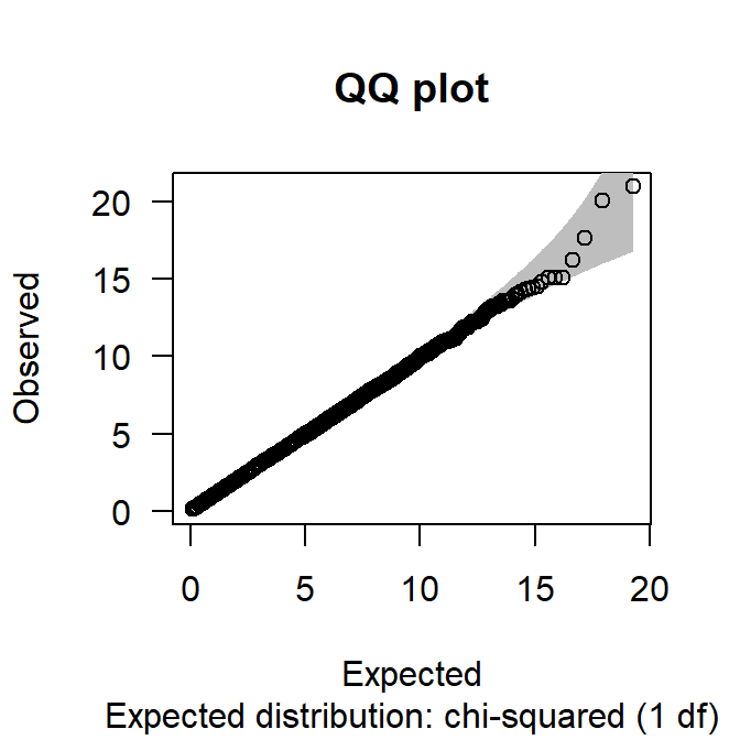
Figure 4.3: QQ-plot corresponding to obesity GWAS data example.
           N      omitted       lambda
88723.000000     0.000000     1.003853
Figure @ref{fig:qqPlot} shows, in particular, that the \(\chi^2\) estimates are not inflated (\(\lambda\) is also close to 1), as all quantile values fall in the confidence bands, meaning that most SNPs are not associated with obesity. In addition, the Figure does not show any top SNP outside the confidence bands. A Q-Q plot with top SNPs outside the confidence bands indicates that those SNPs are truly associated with the disease and, hence, do not follow the null hypothesis. Therefore, the Q-Q plot of our examples reveals no significant SNP associations.
Q-Q plots are used to inspect population stratification. In particular, when population stratification is present, most SNP Q-Q values will be found outside the confidence bands, suggesting that the overall genetic structure of the sample can discriminate differences between subject traits. The \(\lambda\) value is a measure of the degree of inflation. The main source of population stratification that is derived from genomic data is ancestry. Therefore, in the cases of inflated Q-Q plots, it is ancestry differences and not individual SNP differences that explain the differences in the phenotype. Population stratification may be corrected by genomic control, mixed models or EIGENSTRAT method Price et al. (2010). However, the most common approach is to use the inferred ancestry from genomic data as covariates in the association analyses Price et al. (2006). Genome-wide association analysis typically adjusts for population stratification using the PCs on genomic data to infer ancestral differences in the sample. Covariates are easily incorporated in the model of snp.rhs.tests() function.
res.adj <- snp.rhs.tests(obese ~ X1 + X2 + X3 + X4 + X5,
                         data=ob.qc, snp.data=geno.qc)
head(res.adj)
Chi.squared Df p.value
MitoT9699C 2.660902 1 0.1028424This function only computes the additive model, adjusting for the first five genomic PCs. The resulting \(-\log_{10}(P)\)-values of association for each SNP are then extracted
pval.log10 <- -log10(p.value(res.adj))These transformed \(P\)-values are used to create a Manhattan plot to visualize which SNPs are significantly associated with obesity. We use our function manhattanPlot(), although package qqman can also be used.
The function manhattanPlot() can be downloaded as follows:
source("https://raw.githubusercontent.com/isglobal-brge/book_omic_association/master/R/manhattanPlot.R")library(tidyverse)
library(ggplot2)
library(ggrepel)
# Create the required data frame
pvals <- data.frame(SNP=annotation$snp.name,
CHR=annotation$chromosome,
BP=annotation$position,
P=p.value(res.adj))
# missing data is not allowed
pvals <- subset(pvals, !is.na(CHR) & !is.na(P))
manhattanPlot(pvals, color=c("gray90", "gray40"))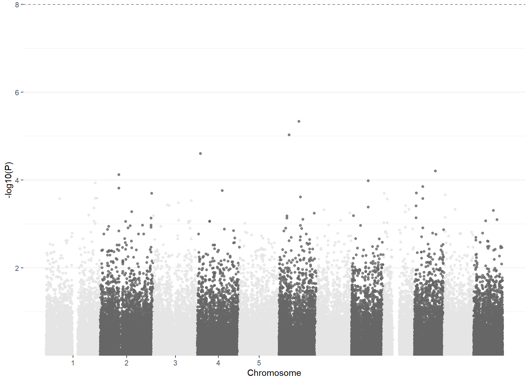
Figure 4.4: Manhattan plot of obesity GWAS data example.
Significance at Bonferroni level is set at \(10^{-7}=0.05/10^5\), as we are testing 100,000 SNPs. The level corresponds to \(-\log_{10}(P)=6.30\). Therefore, we confirm, as expected form the Q-Q plot, that no SNP in our study is significantly associated with obesity, as observed in Figure @ref{fig:manhattan}. It should be noticed that the standard Bonferroni significant level in GWASs is considered as \(5 \times 10^{-8}\) since SNParray data use to contain 500K-1M SNPs (Pe’er et al. 2008).
With our obesity example, we illustrate the common situation of finding no significant associations in small studies (thousands of subjects) with small genomic data (100,000 SNPs). This situation motivates multi-center studies with larger samples sizes, where small effects can be inferred with sufficient power and consistency.
The snpStats package performs association analyses using either codominant or additive models and only provides their p-values. Let us imagine we are interested in using SNPassoc to create the tables with the different genetic models for the most significant SNPs. This can be performed as following. We first select the SNPs that pass a p-value threshold. For instance, \(10^{-5}\) (in real situations it should be the GWAS level \(5 \times 10^{-8}\))
topPvals <- subset(pvals, P<10e-5)
topSNPs <- as.character(topPvals$SNP)
We then export the data into a text file that can be imported into R as a data.frame that can be analyzed using SNPassoc
# subset top SNPs
geno.topSNPs <- geno.qc[, topSNPs]
geno.topSNPs
A SnpMatrix with 2242 rows and 5 columns
Row names: 100 ... 998
Col names: rs10193241 ... rs1935960 # export top SNPs
write.SnpMatrix(geno.topSNPs, file="topSNPs.txt")[1] 2242 5# import top SNPs
ob.top <- read.delim("topSNPs.txt", sep="")
# add phenotypic information(ids are in the same order)
ob.top <- cbind(ob.top, ob.qc)
# prepare data for SNPassoc (SNPs are coded as 0,1,2)
ii <- grep("^rs", names(ob.top))
ob.top.s <- setupSNP(ob.top, colSNPs = ii,
name.genotypes=c(0,1,2))
# run association (all)
WGassociation(obese, ob.top.s) comments codominant dominant recessive overdominant log-additive
rs10193241 - 0.00026 0.19355 0.00005 0.00044 0.00013
rs7349742 - 0.00009 0.01839 0.00004 0.00182 0.00002
rs12201995 - 0.00006 0.00185 0.00011 0.01271 0.00001
rs6931936 - 0.00001 0.00078 0.00002 0.00368 0.00000
rs1935960 - 0.00006 0.74717 0.00001 0.00001 0.00009# run association (one)
association(obese ~ rs10193241, ob.top.s)
SNP: rs10193241  adjusted by:
                0    %   1    %   OR lower upper   p-value  AIC
Codominant
A/A            85  4.9  26  6.5 1.00             2.648e-04 2040
A/B           617 35.5 179 45.1 0.95  0.59  1.52
B/B          1034 59.6 192 48.4 0.61  0.38  0.97
Dominant
A/A            85  4.9  26  6.5 1.00             1.935e-01 2052
A/B-B/B      1651 95.1 371 93.5 0.73  0.47  1.16
Recessive
A/A-A/B       702 40.4 205 51.6 1.00             5.063e-05 2038
B/B          1034 59.6 192 48.4 0.64  0.51  0.79
Overdominant
A/A-B/B      1119 64.5 218 54.9 1.00             4.365e-04 2042
A/B           617 35.5 179 45.1 1.49  1.19  1.86
log-Additive
0,1,2        1736 81.4 397 18.6 0.71  0.59  0.84 1.313e-04 2039