2 Bioconductor
This chapter offers a summary of the main data structures that are implemented in Bioconductor for dealing with genomic, transcriptomic and epigenomic data data. Omic data is typically composed of three datasets: one containing the actual high-dimensional data of omic variables per individuals, annotation data that specifies the characteristics of the variables and phenotypic information that encodes the subject’s traits of interest, covariates and sampling characteristics. For instance, transcriptomic data is stored in a ExpressionSet object, which is a data structure that contains the transcription values of individuals at each transcription probe, the genomic information for the transcription probes and the phenotypes of the individuals. Specific data is accessed, processed and analyzed with specific functions from diverse packages, conceived as methods acting on the ExpressionSet object. The aim of this chapter is then to introduce the specific omic objects available in Bioconductor. In the following chapters, we will introduce the packages that have been implemented to process and analyze these objects. We finish the chapter by illustrating how to perform genomic annotation which is crucial for interpreting results.
Some of the data we are working with are available at our repository called brgedata. Therefore, I would recommend to install it just executing:
BiocManager::install("isglobal-brge/brgedata")2.1 Bioconductor’s overview
Bioconductor: Analysis and comprehension of high-throughput genomic data
- Statistical analysis: large data, technological artifacts, designed experiments; rigorous
- Comprehension: biological context, visualization, reproducibility
- High-throughput
- Sequencing: RNASeq, ChIPSeq, variants, copy number, …
- Microarrays: expression, SNP, …
- Flow cytometry, proteomics, images, …
Packages, vignettes, work flows
- 1974 software packages (Nov’20); also…
- ‘Annotation’ packages – static data bases of identifier maps, gene models, pathways, etc; e.g., [TxDb.Hsapiens.UCSC.hg19.knownGene][]
- ’Experiment packages – data sets used to illustrate software functionality, e.g., airway
- Discover and navigate via [biocViews][]
- Package ‘landing page’
- Title, author / maintainer, short description, citation, installation instructions, …, download statistics
- All user-visible functions have help pages, most with runnable examples
- ‘Vignettes’ an important feature in Bioconductor – narrative documents illustrating how to use the package, with integrated code
- ‘Release’ (every six months) and ‘devel’ branches
- Support site; videos; recent courses.
- Common Workflows
Package installation and use
A package needs to be installed once, using the instructions on the package landing page (e.g., DESeq2).
source("https://bioconductor.org/biocLite.R")
biocLite(c("DESeq2", "org.Hs.eg.db"))
NEW functions have been created
require(BiocManager)
install("DESeq2")

# or

BiocManager::install("DESeq2")
older versions can be installed by
```r
BiocManager::install("DESeq2", version = "3.8")
```biocLite()andinstall()install Bioconductor and [CRAN][]Github packages can be install by
devtools::install_github("isglobal-brge/SNPassoc")Once installed, the package can be loaded into an R session
library(GenomicRanges)and the help system queried interactively, as outlined above:
help(package="GenomicRanges")
vignette(package="GenomicRanges")
vignette(package="GenomicRanges", "GenomicRangesHOWTOs")
?GRanges
2.2 Bioconductor infrastructures
2.2.1 snpMatrix
SNP array data can be stored in different formats. PLINK binary format is a common and efficient system to store and analyze genotype data. It was developed to analyze data with PLINK software (Purcell et al. 2007) but its efficiency in storing data in binary files has made it one of the standard formats for other software packages, including some in Bioconductor. PLINK stores SNP genomic data, annotation and phenotype information in three different files with extensions .bed, .bim and .fam:
- binary BED file: Contains the genomic SNP data, whose values are encoded in two bits (Homozygous normal 00, Heterozygous 10, Homozygous variant 11, missing 01).
- text BIM file: Contains SNPs annotations. Each row is a SNP and contains six columns: chromosome, SNP name, position in morgans, base-pair coordinates, allele 1 (reference nucleotide), allele 2 (alternative nucleotide).
- text FAM file: Contains the subject’s information. Each row is an individual and contains six variables: the Family identifier (ID), Individual ID, Paternal ID, Maternal ID, Sex (1=male; 2=female; other=unknown), phenotypes. Covariates can be added in additional columns.
PLINK data can be loaded into R with the read.plink() function from snpStats Bioconductor’s package. The function requires the full path for the BED, BIM and FAM files, or only their name when the working directory of R contains the PLINK files.
library(snpStats)
ob.plink <- read.plink(bed = "obesity.bed",
                       bim = "obesity.bim",
                       fam = "obesity.fam")
In case of having the three files with the same name (i.e. obesity.fam, obesity.bim and obesity.bed) the following simplification may be convenient:
snps <- read.plink("obesity") Let us assume we have our PLINK data in folder called “data” at our working directory. Therefore, they can also be loaded by
library(snpStats)
path <- "data"
snps <- read.plink(file.path(path, "obesity"))
names(snps)
[1] "genotypes" "fam" "map" The read.plink() function returns a list with the three fields genotypes, fam and map that correspond to the three uploaded files. The genotypes field contains the genotype data stored in a snpMatrix object (individuals in rows and SNPs in columns).
geno <- snps$genotypes
geno
A SnpMatrix with 2312 rows and 100000 columns
Row names: 100 ... 998
Col names: MitoC3993T ... rs28600179 Genotypes are encoded as raw variables for storage efficiency. While individual values can be extracted with array syntax, manipulation of data is usually performed by methods that act on the complete object. The fam field contains the individual’s information in a data.frame object:
individuals <- snps$fam
head(individuals)
pedigree member father mother sex affected
100 FAM_OB 100 NA NA 1 1
1001 FAM_OB 1001 NA NA 1 1
1004 FAM_OB 1004 NA NA 2 2
1005 FAM_OB 1005 NA NA 1 2
1006 FAM_OB 1006 NA NA 2 1
1008 FAM_OB 1008 NA NA 1 1The map field contains the SNPs annotation in a data.frame:
annotation <- snps$map
head(annotation)
chromosome snp.name cM position allele.1 allele.2
MitoC3993T NA MitoC3993T NA 3993 T C
MitoG4821A NA MitoG4821A NA 4821 A G
MitoG6027A NA MitoG6027A NA 6027 A G
MitoT6153C NA MitoT6153C NA 6153 C T
MitoC7275T NA MitoC7275T NA 7275 T C
MitoT9699C NA MitoT9699C NA 9699 C TSubsetting SNP data requires at least two different operations. For instance, if we are interested in extracting the SNPs of chromosome 1, we need to select those variants in annotation that are located in chromosome 1 and then subset the snpMatrix object as a typical matrix.
annotationChr1 <- annotation[annotation$chromosome == "1" &
                               !is.na(annotation$chromosome), ]
genoChr1 <- geno[, rownames(annotationChr1)]
genoChr1
A SnpMatrix with 2312 rows and 7721 columns
Row names: 100 ... 998
Col names: rs12354060 ... rs7527472 Subsetting samples follow a similar pattern. Suppose we want to select the genotypes of the control individuals. Case-control status is often encoded in the FAM file and therefore uploaded in the fam field. In our example, controls are coded with 1 and cases with 2 in the variable “affected” of individuals. Therefore, the genotypes of the control samples are extracted by
individualsCtrl <- individuals[individuals$affected == 1, ]
genoCtrl <- geno[rownames(individualsCtrl), ]
genoCtrl
A SnpMatrix with 1587 rows and 100000 columns
Row names: 100 ... 998
Col names: MitoC3993T ... rs28600179 2.2.2 ExpressionSet
ExpressionSetwas one of the first implementations of Bioconductor to manage omic experiments. This figure illustrates how it is implemented
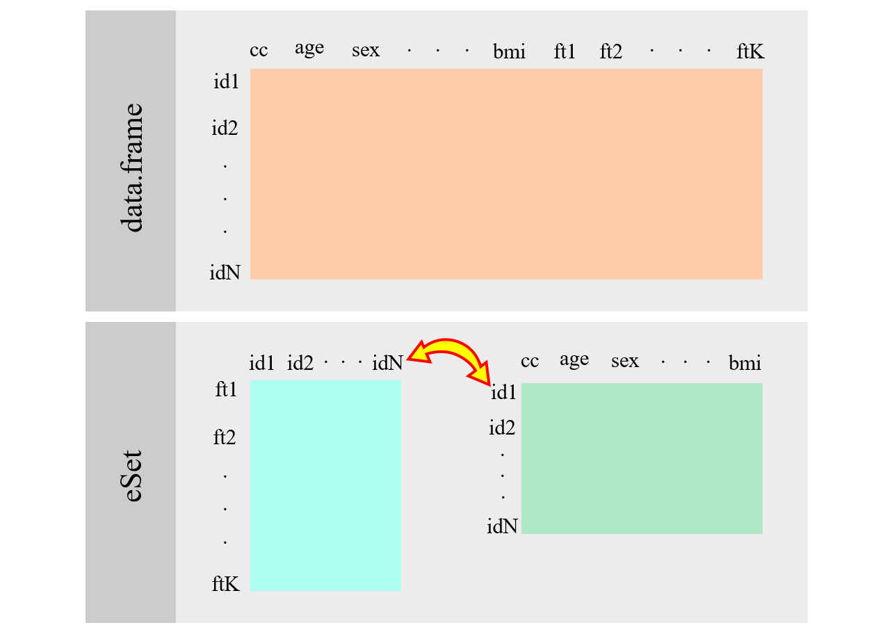
Figure 2.1: ExpressionSet scheme.
Although its use is discouraged in Bioconductor’s guidelines for the development of current and future packages, most publicly available data is available in this structure while future packages are still required to be able to upload and operate with it. The GEO repository contains thousands of transcriptomic experiments that are available in ExpressionSet format. Data available in GEO repository can be donwloaded into R as an ExpressionSet using GEOquery package. Let us donwload the experiment with accession number GSE63061 from the GEO website
library(GEOquery)
gsm.expr <- getGEO("GSE63061", destdir = ".")[[1]]
gsm.expr
ExpressionSet (storageMode: lockedEnvironment)
assayData: 32049 features, 388 samples
element names: exprs
protocolData: none
phenoData
sampleNames: GSM1539409 GSM1539410 ... GSM1539796 (388 total)
varLabels: title geo_accession ... tissue:ch1 (40 total)
varMetadata: labelDescription
featureData
featureNames: ILMN_1343291 ILMN_1343295 ... ILMN_3311190 (32049 total)
fvarLabels: ID Species ... GB_ACC (30 total)
fvarMetadata: Column Description labelDescription
experimentData: use 'experimentData(object)'
pubMedIds: 26343147
Annotation: GPL10558 gsm.expr is an object of class ExpressionSet that has three main slots. Transcriptomic data is stored in the assayData slot, phenotypes are in phenoData and probe annotation in featuredData. There are three other slots protocolData, experimentData and annotation that specify equipment-generated information about protocols, resulting publications and the platform on which the samples were assayed. Methods are implemented to extract the data from each slot of the object. For instance exprs extracts the transcriptomic data in a matrix where subjects are columns and probes are rows
expr <- exprs(gsm.expr)
dim(expr)
[1] 32049 388expr[1:5,1:5] GSM1539409 GSM1539410 GSM1539411 GSM1539412 GSM1539413
ILMN_1343291 12.552807 12.711459 13.088393 12.643831 13.098389
ILMN_1343295 10.101556 9.776015 9.594397 10.126782 10.223301
ILMN_1651209 6.084671 6.255012 6.160485 6.109219 6.069960
ILMN_1651210 6.068805 6.016468 6.024322 6.016118 6.056163
ILMN_1651221 6.121060 6.173167 6.039552 6.111306 6.089542phenoData() retrieves the subjects’ phenotypes in an AnnotatedDataFrame object which is converted to a data.frame by the function pData()
#get phenotype data
pheno <- phenoData(gsm.expr)
pheno
An object of class 'AnnotatedDataFrame'
sampleNames: GSM1539409 GSM1539410 ... GSM1539796 (388
total)
varLabels: title geo_accession ... tissue:ch1 (40
total)
varMetadata: labelDescriptionphenoDataFrame <- pData(gsm.expr)
phenoDataFrame[1:5,1:4] title geo_accession status
GSM1539409 7196843065_F GSM1539409 Public on Aug 05 2015
GSM1539410 7196843076_G GSM1539410 Public on Aug 05 2015
GSM1539411 7196843068_B GSM1539411 Public on Aug 05 2015
GSM1539412 7196843063_B GSM1539412 Public on Aug 05 2015
GSM1539413 7196843065_L GSM1539413 Public on Aug 05 2015
submission_date
GSM1539409 Nov 06 2014
GSM1539410 Nov 06 2014
GSM1539411 Nov 06 2014
GSM1539412 Nov 06 2014
GSM1539413 Nov 06 2014#Alzheimer's case control variable
table(phenoDataFrame$characteristics_ch1)
            status: AD status: borderline MCI
                   139                      3
           status: CTL      status: CTL to AD
                   134                      1
           status: MCI     status: MCI to CTL
                   109                      1
         status: OTHER
                     1
Finally the fData() function gets the probes’ annotationin a data.frame
probes <- fData(gsm.expr)
probes[1:5, 1:5]
ID Species Source Search_Key Transcript
ILMN_1343291 ILMN_1343291 Homo sapiens RefSeq NM_001402.4 ILMN_5311
ILMN_1343295 ILMN_1343295 Homo sapiens RefSeq ILMN_27206
ILMN_1651209 ILMN_1651209 Homo sapiens RefSeq NM_182838.1 ILMN_8692
ILMN_1651210 ILMN_1651210 Homo sapiens RefSeq XM_941691.1 ILMN_138115
ILMN_1651221 ILMN_1651221 Homo sapiens RefSeq XM_926225.1 ILMN_335282.2.3 SummarizedExperiment
The SummarizedExperiment class is a comprehensive data structure that can be used to store expression and methylation data from microarrays or read counts from RNA-seq experiments, among others. A SummarizedExperiment object contains slots for one or more datasets, feature annotation (e.g. genes, transcripts, SNPs, CpGs), individual phenotypes and experimental details, such as laboratory and experimental protocols. In a SummarizedExperiment, the rows of omic data are features and columns are subjects.

SummarizedExperiment
Information is coordinated across the object’s slots. For instance, subsetting samples in the assay matrix automatically subsets them in the phenotype metadata. A SummarizedExperimentobject is easily manipulated and constitutes the input and output of many of Bioconductor’s methods.
Data is retrieved from a SummarizedExperiment by using specific methods or accessors. We illustrate the functions with brge_methy which includes real methylation data and is available from the Bioconductor’s brgedata package. The data is made available by loading of the package
library(brgedata)
brge_methy
class: GenomicRatioSet
dim: 392277 20
metadata(0):
assays(1): Beta
rownames(392277): cg13869341 cg24669183 ... cg26251715
cg25640065
rowData names(14): Forward_Sequence SourceSeq ...
Regulatory_Feature_Group DHS
colnames(20): x0017 x0043 ... x0077 x0079
colData names(9): age sex ... Mono Neu
Annotation
array: IlluminaHumanMethylation450k
annotation: ilmn12.hg19
Preprocessing
Method: NA
minfi version: NA
Manifest version: NAextends("GenomicRatioSet")[1] "GenomicRatioSet" "RangedSummarizedExperiment"
[3] "SummarizedExperiment" "Vector"
[5] "Annotated" "vector_OR_Vector" The function extends() shows that the data has been encoded in an object of GenomicRatioSet class, which is an extension of the more primitive classes RangedSummarizedExperiment and SummarizedExperiment. brge_methy illustrates a typical object within Bioconductor’s framework, as it is a structure that inherits different types of classes in an established hierarchy. For each class, there are specific methods which are properly inherited across classes. For instance, in our example, SummarizedExperiment is brge_methy’s most primitive omic class and, therefore, all the methods of SummarizedExperiment apply to it. In particular, the methylation data that is stored in the object can be extracted with the function assay()
betas <- assay(brge_methy)
betas[1:5, 1:4]
x0017 x0043 x0036 x0041
cg13869341 0.90331003 0.90082827 0.8543610 0.84231205
cg24669183 0.86349463 0.84009629 0.8741255 0.85122181
cg15560884 0.65986032 0.69634338 0.6931083 0.69752294
cg01014490 0.01448404 0.01509478 0.0163614 0.01322362
cg17505339 0.92176287 0.92060149 0.9101060 0.93249167The assay slot of a SummarizedExperiment object can contain any type of data (i.e. numeric, character, factor…), structure or large on-disk representations, such as a HDF5Array. Feature annotation data is accessed with the function rowData():
rowData(brge_methy)[,2:5]DataFrame with 392277 rows and 4 columns
SourceSeq
<character>
cg13869341 CCGGTGGCTGGCCACTCTGCTAGAGTCCATCCGCCAAGCTGGGGGCATCG
cg24669183 TCACCGCCTTGACAGCTTTGCAGAGTGCTGCTCAGGTATTCTGCAAGACG
cg15560884 CGCGTAAACAAGGGAAGCTGAGTAATTGTATGTTCAAATACTTGCAAAAC
cg01014490 TCAGAACTCGCGGTGGGGGCTGCTGGTTCTTCCAGGAGCGCGCATGAGCG
cg17505339 AAACAAACAAAGATATCAAGCCACAGATTCAAAGTGCTATAAACTCCACG
... ...
cg04964672 CGGCGGCTTTCCACGCTGCGGCTTGGAGTGGTCCTTGTTTAGATTCCTTT
cg01086462 CGCAGGTATGGTGTACATTAAGCAGGCAGGGTCAATCAGGGATGGTCTAT
cg02233183 CAAAATGAATGAAATTTACAAACCCAGCAGCCAATAGATCTCCAGAGTCG
cg26251715 CGCTGGTTGTCCAGGCTGGAATGCAATGGTGCAATGTCCGCTCACTCCAA
cg25640065 CGGGGCAGGGGTCCGTAACTGCAGCCCTCCATGCCTGAGCCCCCCACCCC
Random_Loci Methyl27_Loci genes
<character> <character> <character>
cg13869341 WASH5P
cg24669183
cg15560884
cg01014490
cg17505339
... ... ... ...
cg04964672
cg01086462
cg02233183 NLGN4Y;NLGN4Y
cg26251715 TTTY14
cg25640065 which returns a data.frame object. In our example, it contains the sequences and the genes associated with the CpG probes, among other information.
2.2.4 Genomic Ranges (GRanges)
The Bioconductor’s package GenomicRanges aims to represent and manipulate the genomic annotation of molecular omic data under a reference genome. It contains functions to select specific regions and perform operations with them (Lawrence et al. 2013). Objects of GRanges class are important to annotate and manipulate genomic, transcriptomic and methylomic data. In particular, they are used in conjunction with SummarizedExperiment, within the RangedSummarizedExperiment class that is explained in the following section.
Annotation data refers to the characteristics of the variables in the high-dimensional data set. In particular for omic data relative to DNA structure and function, each variable may be given a location in a reference genome. While not two genomes are identical, the construction of a reference genome allows the mapping of specific characteristics of individual genomes to a common ground where they can be compared. The reference genome defines a coordinate system: “chromosome id” and “position along the chromosome.” For instance, a position such as chr10:4567-5671 would represent the 4567th to the 5671st base pair on the reference’s chromosome 10.
The main functionalities implemented GenomicRanges are methods on GRanges objects. Objects are created by the function GRanges, minimum requirements are the genomic positions given by the chromosome seqnames and base pair coordinates ranges. Other metadata (e.g. variables) can be added to provide further information about each segment.
We illustrate GenomicRanges creating 8 segments on either chr1 or chr2, each with defined start and end points. We add strand information, passed through the argument strand, to indicate the direction of each sequence. We also add a hypothetical variable disease that indicates whether asthma or obesity have been associated with each interval
library(GenomicRanges)
gr <- GRanges(seqnames=c(rep("chr1", 4), rep("chr2", 4)),
              ranges = IRanges(start = c(1000, 1800, 5300, 7900,
                                         1300, 2100, 3400, 6700),
                               end =c(2200, 3900, 5400, 8100,
                                      2600, 3300, 4460, 6850)),
              strand = rep(c("+", "-"), 4),
              disease = c(rep("Asthma",4), rep("Obesity",4)))
gr
GRanges object with 8 ranges and 1 metadata column:
seqnames ranges strand | disease
<Rle> <IRanges> <Rle> | <character>
[1] chr1 1000-2200 + | Asthma
[2] chr1 1800-3900 - | Asthma
[3] chr1 5300-5400 + | Asthma
[4] chr1 7900-8100 - | Asthma
[5] chr2 1300-2600 + | Obesity
[6] chr2 2100-3300 - | Obesity
[7] chr2 3400-4460 + | Obesity
[8] chr2 6700-6850 - | Obesity
-------
seqinfo: 2 sequences from an unspecified genome; no seqlengthsgr is our constructed object of class GRanges. The object responds to the usual array and subset extraction given by squared parentheses
gr[1]GRanges object with 1 range and 1 metadata column:
seqnames ranges strand | disease
<Rle> <IRanges> <Rle> | <character>
[1] chr1 1000-2200 + | Asthma
-------
seqinfo: 2 sequences from an unspecified genome; no seqlengthsHowever, there are also specific functions to access and modify information. For instance, seqnames() extract the chromosomes defined in our examples, whose first element can be redefined accordingly:
seqnames(gr)factor-Rle of length 8 with 2 runs
Lengths: 4 4
Values : chr1 chr2
Levels(2): chr1 chr2seqnames(gr)[1] <- "chr2"
grGRanges object with 8 ranges and 1 metadata column:
seqnames ranges strand | disease
<Rle> <IRanges> <Rle> | <character>
[1] chr2 1000-2200 + | Asthma
[2] chr1 1800-3900 - | Asthma
[3] chr1 5300-5400 + | Asthma
[4] chr1 7900-8100 - | Asthma
[5] chr2 1300-2600 + | Obesity
[6] chr2 2100-3300 - | Obesity
[7] chr2 3400-4460 + | Obesity
[8] chr2 6700-6850 - | Obesity
-------
seqinfo: 2 sequences from an unspecified genome; no seqlengthsThis is important to annotation using different system. NCBI encodes chromosomes as 1, 2, 3, …; while UCSC uses chr1, chr2, … The chromosome style can be changed using
seqlevelsStyle(gr) <- "NCBI"
gr
GRanges object with 8 ranges and 1 metadata column:
seqnames ranges strand | disease
<Rle> <IRanges> <Rle> | <character>
[1] 2 1000-2200 + | Asthma
[2] 1 1800-3900 - | Asthma
[3] 1 5300-5400 + | Asthma
[4] 1 7900-8100 - | Asthma
[5] 2 1300-2600 + | Obesity
[6] 2 2100-3300 - | Obesity
[7] 2 3400-4460 + | Obesity
[8] 2 6700-6850 - | Obesity
-------
seqinfo: 2 sequences from an unspecified genome; no seqlengthsLet’s us write back the UCSC style
seqlevelsStyle(gr) <- "UCSC"
gr
GRanges object with 8 ranges and 1 metadata column:
seqnames ranges strand | disease
<Rle> <IRanges> <Rle> | <character>
[1] chr2 1000-2200 + | Asthma
[2] chr1 1800-3900 - | Asthma
[3] chr1 5300-5400 + | Asthma
[4] chr1 7900-8100 - | Asthma
[5] chr2 1300-2600 + | Obesity
[6] chr2 2100-3300 - | Obesity
[7] chr2 3400-4460 + | Obesity
[8] chr2 6700-6850 - | Obesity
-------
seqinfo: 2 sequences from an unspecified genome; no seqlengthsAdditional information can be added to the current object as a new field of a list
gr$gene_id <- paste0("Gene", 1:8)
gr
GRanges object with 8 ranges and 2 metadata columns:
seqnames ranges strand | disease gene_id
<Rle> <IRanges> <Rle> | <character> <character>
[1] chr2 1000-2200 + | Asthma Gene1
[2] chr1 1800-3900 - | Asthma Gene2
[3] chr1 5300-5400 + | Asthma Gene3
[4] chr1 7900-8100 - | Asthma Gene4
[5] chr2 1300-2600 + | Obesity Gene5
[6] chr2 2100-3300 - | Obesity Gene6
[7] chr2 3400-4460 + | Obesity Gene7
[8] chr2 6700-6850 - | Obesity Gene8
-------
seqinfo: 2 sequences from an unspecified genome; no seqlengthsGenomicRanges provides different methods to perform arithmetic with the ranges, see ?GRanges for a full list. For instance, with shift() an interval is moved a given base-pair distance and with flank() the interval is stretched
#shift: move all intervals 10 base pair towards the end
shift(gr, 10)
GRanges object with 8 ranges and 2 metadata columns:
seqnames ranges strand | disease gene_id
<Rle> <IRanges> <Rle> | <character> <character>
[1] chr2 1010-2210 + | Asthma Gene1
[2] chr1 1810-3910 - | Asthma Gene2
[3] chr1 5310-5410 + | Asthma Gene3
[4] chr1 7910-8110 - | Asthma Gene4
[5] chr2 1310-2610 + | Obesity Gene5
[6] chr2 2110-3310 - | Obesity Gene6
[7] chr2 3410-4470 + | Obesity Gene7
[8] chr2 6710-6860 - | Obesity Gene8
-------
seqinfo: 2 sequences from an unspecified genome; no seqlengths#shift: move each intervals individually
shift(gr, seq(10,100, length=8))GRanges object with 8 ranges and 2 metadata columns:
seqnames ranges strand | disease gene_id
<Rle> <IRanges> <Rle> | <character> <character>
[1] chr2 1010-2210 + | Asthma Gene1
[2] chr1 1822-3922 - | Asthma Gene2
[3] chr1 5335-5435 + | Asthma Gene3
[4] chr1 7948-8148 - | Asthma Gene4
[5] chr2 1361-2661 + | Obesity Gene5
[6] chr2 2174-3374 - | Obesity Gene6
[7] chr2 3487-4547 + | Obesity Gene7
[8] chr2 6800-6950 - | Obesity Gene8
-------
seqinfo: 2 sequences from an unspecified genome; no seqlengths#flank: recover regions next to the input set.
# For a 50 base stretch upstream (negative value for
# downstream)
flank(gr, 50)GRanges object with 8 ranges and 2 metadata columns:
seqnames ranges strand | disease gene_id
<Rle> <IRanges> <Rle> | <character> <character>
[1] chr2 950-999 + | Asthma Gene1
[2] chr1 3901-3950 - | Asthma Gene2
[3] chr1 5250-5299 + | Asthma Gene3
[4] chr1 8101-8150 - | Asthma Gene4
[5] chr2 1250-1299 + | Obesity Gene5
[6] chr2 3301-3350 - | Obesity Gene6
[7] chr2 3350-3399 + | Obesity Gene7
[8] chr2 6851-6900 - | Obesity Gene8
-------
seqinfo: 2 sequences from an unspecified genome; no seqlengthsGenomicRanges also includes methods for aggregating and summarizing GRangesobjects. The functions reduce(), disjoint() and coverage() are most useful. disjoin(), for instance, reduces the intervals into the smallest set of unique, non-overlapping pieces that make up the original object. It is strand-specific by default, but this can be avoided with ignore.strand=TRUE.
disjoin(gr, ignore.strand=TRUE)GRanges object with 10 ranges and 0 metadata columns:
seqnames ranges strand
<Rle> <IRanges> <Rle>
[1] chr1 1800-3900 *
[2] chr1 5300-5400 *
[3] chr1 7900-8100 *
[4] chr2 1000-1299 *
[5] chr2 1300-2099 *
[6] chr2 2100-2200 *
[7] chr2 2201-2600 *
[8] chr2 2601-3300 *
[9] chr2 3400-4460 *
[10] chr2 6700-6850 *
-------
seqinfo: 2 sequences from an unspecified genome; no seqlengthsreduce() creates the smallest range set of unique, non-overlapping intervals. Strand information is also taken into account by default and can also be turned off
reduce(gr, ignore.strand=TRUE)GRanges object with 6 ranges and 0 metadata columns:
seqnames ranges strand
<Rle> <IRanges> <Rle>
[1] chr1 1800-3900 *
[2] chr1 5300-5400 *
[3] chr1 7900-8100 *
[4] chr2 1000-3300 *
[5] chr2 3400-4460 *
[6] chr2 6700-6850 *
-------
seqinfo: 2 sequences from an unspecified genome; no seqlengthscoverage() summarizes the times each base is covered by an interval
coverage(gr)RleList of length 2
$chr1
integer-Rle of length 8100 with 6 runs
Lengths: 1799 2101 1399 101 2499 201
Values : 0 1 0 1 0 1
$chr2
integer-Rle of length 6850 with 10 runs
Lengths: 999 300 800 101 400 700 99 1061 2239 151
Values : 0 1 2 3 2 1 0 1 0 1It is also possible to perform operations between two different GRanges objects. For instance, one may be interested in knowing the intervals that overlap with a targeted region:
target <- GRanges(seqnames="chr1",
                  range=IRanges(start=1200, 4000))
target
GRanges object with 1 range and 0 metadata columns:
seqnames ranges strand
<Rle> <IRanges> <Rle>
[1] chr1 1200-4000 *
-------
seqinfo: 1 sequence from an unspecified genome; no seqlengthsgr.ov <- findOverlaps(target, gr)
gr.ovHits object with 1 hit and 0 metadata columns:
queryHits subjectHits
<integer> <integer>
[1] 1 2
-------
queryLength: 1 / subjectLength: 8To recover the overlapping intervals between gr and target we can run
gr[subjectHits(gr.ov)]GRanges object with 1 range and 2 metadata columns:
seqnames ranges strand | disease gene_id
<Rle> <IRanges> <Rle> | <character> <character>
[1] chr1 1800-3900 - | Asthma Gene2
-------
seqinfo: 2 sequences from an unspecified genome; no seqlengthsor
subsetByOverlaps(gr, target)GRanges object with 1 range and 2 metadata columns:
seqnames ranges strand | disease gene_id
<Rle> <IRanges> <Rle> | <character> <character>
[1] chr1 1800-3900 - | Asthma Gene2
-------
seqinfo: 2 sequences from an unspecified genome; no seqlengthsOther operations can be found here.
2.2.5 RangedSummarizedExperiment
SummarizedExperiment is extended to RangedSummarizedExperiment, a child class that contains the annotation data of the features in a GenomicRanges object. In our epigenomic example, the second most primitive class of brge_methy object with omic functionality, after SummarizedExperiment, is RangedSummarizedExperiment. Annotation data, with variable names given by
names(rowData(brge_methy)) [1] "Forward_Sequence" "SourceSeq"
[3] "Random_Loci" "Methyl27_Loci"
[5] "genes" "UCSC_RefGene_Accession"
[7] "group" "Phantom"
[9] "DMR" "Enhancer"
[11] "HMM_Island" "Regulatory_Feature_Name"
[13] "Regulatory_Feature_Group" "DHS" can be obtained in a GRanges object, for a given variable. For instance, metadata of CpG genomic annotation and neighboring genes is obtained using array syntax
rowRanges(brge_methy)[, "genes"]GRanges object with 392277 ranges and 1 metadata column:
seqnames ranges strand | genes
<Rle> <IRanges> <Rle> | <character>
cg13869341 chr1 15865 * | WASH5P
cg24669183 chr1 534242 * |
cg15560884 chr1 710097 * |
cg01014490 chr1 714177 * |
cg17505339 chr1 720865 * |
... ... ... ... . ...
cg04964672 chrY 7428198 * |
cg01086462 chrY 7429349 * |
cg02233183 chrY 16634382 * | NLGN4Y;NLGN4Y
cg26251715 chrY 21236229 * | TTTY14
cg25640065 chrY 23569324 * |
-------
seqinfo: 24 sequences from an unspecified genome; no seqlengthsSubject data can be accessed entirely in a single data.frame or a variable at the time. The entire subject (phenotype) information is retrieved with the function colData():
colData(brge_methy)DataFrame with 20 rows and 9 columns
age sex NK Bcell CD4T CD8T
<numeric> <factor> <numeric> <numeric> <numeric> <numeric>
x0017 4 Female -5.81386e-19 0.1735078 0.20406869 0.1009741
x0043 4 Female 1.64826e-03 0.1820172 0.16171272 0.1287722
x0036 4 Male 1.13186e-02 0.1690173 0.15546368 0.1277417
x0041 4 Female 8.50822e-03 0.0697158 0.00732789 0.0321861
x0032 4 Male 0.00000e+00 0.1139780 0.22230399 0.0216090
... ... ... ... ... ... ...
x0018 4 Female 0.0170284 0.0781698 0.112735 0.06796816
x0057 4 Female 0.0000000 0.0797774 0.111072 0.00910489
x0061 4 Female 0.0000000 0.1640266 0.224203 0.13125212
x0077 4 Female 0.0000000 0.1122731 0.168056 0.07840593
x0079 4 Female 0.0120148 0.0913650 0.205830 0.11475389
Eos Mono Neu
<numeric> <numeric> <numeric>
x0017 0.00000e+00 0.0385654 0.490936
x0043 0.00000e+00 0.0499542 0.491822
x0036 0.00000e+00 0.1027105 0.459632
x0041 0.00000e+00 0.0718280 0.807749
x0032 2.60504e-18 0.0567246 0.575614
... ... ... ...
x0018 8.37770e-03 0.0579535 0.658600
x0057 4.61887e-18 0.1015260 0.686010
x0061 8.51074e-03 0.0382647 0.429575
x0077 6.13397e-02 0.0583411 0.515284
x0079 0.00000e+00 0.0750535 0.513597The list symbol $ can be used, for instance, to obtain the sex of the individuals
brge_methy$sex [1] Female Female Male Female Male Male Male Male Male
[10] Male Female Female Female Male Male Female Female Female
[19] Female Female
Levels: Female MaleSubsetting the entire structure is also possible following the usual array syntax. For example, we can select only males from the brge_methy dataset
brge_methy[, brge_methy$sex == "male"]class: GenomicRatioSet
dim: 392277 0
metadata(0):
assays(1): Beta
rownames(392277): cg13869341 cg24669183 ... cg26251715
cg25640065
rowData names(14): Forward_Sequence SourceSeq ...
Regulatory_Feature_Group DHS
colnames(0):
colData names(9): age sex ... Mono Neu
Annotation
array: IlluminaHumanMethylation450k
annotation: ilmn12.hg19
Preprocessing
Method: NA
minfi version: NA
Manifest version: NAThe metadata() function retrieves experimental data
metadata(brge_methy)list()which in our case is empty.
2.3 Annotation
2.4 annotate package
Bioconductor distributes annotation packages for a wide range
of gene expression microarrays and RNA-seq data. The annotate
package is one way to use this annotation information. This code loads the annotate package and the databases for the Gene Ontology and one of the Affymetrix human microarray chips.
library(annotate)
library(hgu95av2.db)
library(GO.db)
The databases are queried with get() or mget() for multiple
queries:
get("32972_at", envir=hgu95av2GENENAME)[1] "NADPH oxidase 1"mget(c("738_at", "40840_at", "32972_at"),
envir=hgu95av2GENENAME)$`738_at`
[1] "5'-nucleotidase, cytosolic II"
$`40840_at`
[1] "peptidylprolyl isomerase F"
$`32972_at`
[1] "NADPH oxidase 1"The name of the availabe information in a Bioconductor database (ended by .db, for instance org.Hs.eg.db) can be retreived by using columns():
columns(hgu95av2.db) [1] "ACCNUM" "ALIAS" "ENSEMBL" "ENSEMBLPROT"
[5] "ENSEMBLTRANS" "ENTREZID" "ENZYME" "EVIDENCE"
[9] "EVIDENCEALL" "GENENAME" "GO" "GOALL"
[13] "IPI" "MAP" "OMIM" "ONTOLOGY"
[17] "ONTOLOGYALL" "PATH" "PFAM" "PMID"
[21] "PROBEID" "PROSITE" "REFSEQ" "SYMBOL"
[25] "UCSCKG" "UNIGENE" "UNIPROT" The GO terms can be managed by
go <- get("738_at", envir=hgu95av2GO)
names(go)
[1] "GO:0006195" "GO:0016311" "GO:0017144" "GO:0046040" "GO:0046085"
[6] "GO:0005829" "GO:0000166" "GO:0005515" "GO:0008253" "GO:0046872"get("GO:0009117", envir=GOTERM)GOID: GO:0009117
Term: nucleotide metabolic process
Ontology: BP
Definition: The chemical reactions and pathways involving a
nucleotide, a nucleoside that is esterified with
(ortho)phosphate or an oligophosphate at any hydroxyl
group on the glycose moiety; may be mono-, di- or
triphosphate; this definition includes cyclic nucleotides
(nucleoside cyclic phosphates).
Synonym: nucleotide metabolismThere are multiple annotated databases in Bioconductor that can be found here: annotated data bases. For example
require(org.Hs.eg.db)
columns(org.Hs.eg.db)
[1] "ACCNUM" "ALIAS" "ENSEMBL" "ENSEMBLPROT"
[5] "ENSEMBLTRANS" "ENTREZID" "ENZYME" "EVIDENCE"
[9] "EVIDENCEALL" "GENENAME" "GO" "GOALL"
[13] "IPI" "MAP" "OMIM" "ONTOLOGY"
[17] "ONTOLOGYALL" "PATH" "PFAM" "PMID"
[21] "PROSITE" "REFSEQ" "SYMBOL" "UCSCKG"
[25] "UNIGENE" "UNIPROT" # get the gene symbol
get("9726", envir=org.Hs.egSYMBOL)[1] "ZNF646"2.5 BioMart
BioMart is a query-oriented data management system developed jointly by the European Bioinformatics Institute (EBI) and Cold Spring Harbor Laboratory (CSHL).
biomaRt is an R interface to BioMart systems, in particular
to Ensembl. Ensembl is a joint project between EMBL - European Bioinformatics Institute (EBI) and the Wellcome Trust Sanger Institute (WTSI) to develop a software system which produces and maintains automatic annotation on selected eukaryotic genomes. There are several databases that can be queried:
require(biomaRt)
head(listMarts())
biomart version
1 ENSEMBL_MART_ENSEMBL Ensembl Genes 101
2 ENSEMBL_MART_MOUSE Mouse strains 101
3 ENSEMBL_MART_SNP Ensembl Variation 101
4 ENSEMBL_MART_FUNCGEN Ensembl Regulation 101After selecting a database (e.g., ensembl) we select a dataset:
mart <- useMart(biomart="ensembl")
listDatasets(mart)[1:10,]
dataset
1 acalliptera_gene_ensembl
2 acarolinensis_gene_ensembl
3 acchrysaetos_gene_ensembl
4 acitrinellus_gene_ensembl
5 amelanoleuca_gene_ensembl
6 amexicanus_gene_ensembl
7 ampachon_gene_ensembl
8 anancymaae_gene_ensembl
9 aplatyrhynchos_gene_ensembl
10 applatyrhynchos_gene_ensembl
description
1 Eastern happy genes (fAstCal1.2)
2 Anole lizard genes (AnoCar2.0)
3 Golden eagle genes (bAquChr1.2)
4 Midas cichlid genes (Midas_v5)
5 Panda genes (ailMel1)
6 Mexican tetra genes (Astyanax_mexicanus-2.0)
7 Pachon cavefish genes (Astyanax_mexicanus-1.0.2)
8 Ma's night monkey genes (Anan_2.0)
9 Mallard genes (ASM874695v1)
10 Duck genes (CAU_duck1.0)
version
1 fAstCal1.2
2 AnoCar2.0
3 bAquChr1.2
4 Midas_v5
5 ailMel1
6 Astyanax_mexicanus-2.0
7 Astyanax_mexicanus-1.0.2
8 Anan_2.0
9 ASM874695v1
10 CAU_duck1.0After selecting a dataset (e.g., hsapiens_gene_ensembl) we select the attributes we are interested in:
mart  <- useMart(biomart="ensembl",
                 dataset="hsapiens_gene_ensembl")
listAttributes(mart)[1:10,]
name description
1 ensembl_gene_id Gene stable ID
2 ensembl_gene_id_version Gene stable ID version
3 ensembl_transcript_id Transcript stable ID
4 ensembl_transcript_id_version Transcript stable ID version
5 ensembl_peptide_id Protein stable ID
6 ensembl_peptide_id_version Protein stable ID version
7 ensembl_exon_id Exon stable ID
8 description Gene description
9 chromosome_name Chromosome/scaffold name
10 start_position Gene start (bp)
page
1 feature_page
2 feature_page
3 feature_page
4 feature_page
5 feature_page
6 feature_page
7 feature_page
8 feature_page
9 feature_page
10 feature_pageNOTE: sometimes the host is not working. If so, try host=“www.ensembl.org” in the useMart function.
After selecting the dataset we can make different types of queries:
- Query 1: We could look for all the transcripts contained in the gene
7791(entrez id):
tx <- getBM(attributes="ensembl_transcript_id",
            filters="entrezgene_id",
            values="7791", mart=mart)
tx
ensembl_transcript_id
1 ENST00000322764
2 ENST00000449630
3 ENST00000468083
4 ENST00000457235
5 ENST00000354434
6 ENST00000392910
7 ENST00000477373
8 ENST00000436448
9 ENST00000446634
10 ENST00000497119
11 ENST00000644808
12 ENST00000644767
13 ENST00000645428
14 ENST00000643962
15 ENST00000642783
16 ENST00000644791
17 ENST00000647142
18 ENST00000645637
19 ENST00000646695
20 ENST00000647126- Query 2: We could look for chromosome, position and gene name of a list of genes (entrez id):
genes <- c("79699", "7791", "23140", "26009")
tx <- getBM(attributes=c("chromosome_name", "start_position",
                         "hgnc_symbol"),
            filters="entrezgene_id",
            values=genes, mart=mart)
tx
chromosome_name start_position hgnc_symbol
1 17 4004445 ZZEF1
2 1 77562416 ZZZ3
3 7 143381295 ZYX
4 CHR_HG708_PATCH 143381295 ZYX
5 1 52726453 ZYG11B- Query 3: We could look for chromosome, position and gene name of a list of genes (ENSEMBL):
genes <- c("ENSG00000074755")
tx <- getBM(attributes=c("chromosome_name", "start_position",
                         "hgnc_symbol"),
            filters="ensembl_gene_id",
            values=genes, mart=mart)
tx
chromosome_name start_position hgnc_symbol
1 17 4004445 ZZEF1- Query 4: Homology.
getLDS()combines two data marts, for example to homologous genes in other species. We can look up the mouse equivalents of a particular Affy transcript, or of the NOX1 gene.
human <- useMart("ensembl", dataset = "hsapiens_gene_ensembl")
mouse <- useMart("ensembl", dataset = "mmusculus_gene_ensembl")
getLDS(attributes = c("hgnc_symbol","chromosome_name",
       "start_position"),
       filters = "hgnc_symbol", values = "NOX1",
       mart = human,
       attributesL = c("external_gene_name", "chromosome_name",
       "start_position"),
       martL = mouse)
HGNC.symbol Chromosome.scaffold.name Gene.start..bp. Gene.name
1 NOX1 X 100843324 Nox1
Chromosome.scaffold.name.1 Gene.start..bp..1
1 X 1340864212.6 Annotate SNPs
We had a set of 100 SNPs without chromosome and genomic position information. We need to know the gene that those SNPs belong to.
load("data/snpsList.Rdata")
length(snpsList)
[1] 100head(snpsList)[1] "rs1932919" "rs6849766" "rs11246756" "rs7184849" "rs308857"
[6] "rs16990309"A hand-search (Genome Browser - ) would be easy but tedious, so we want an automated approach.
Rcan be used to carry out the entire analysis. That is, GWAS, annotation and post-GWAS. The annotation can be set by connectingRwith Biomart:
snpmart <- useMart("ENSEMBL_MART_SNP", dataset = "hsapiens_snp")Use
listAttributes()to get valid attribute names.Use
listFilters()to get valid filter names.
head(listAttributes(snpmart)) name description
1 refsnp_id Variant name
2 refsnp_source Variant source
3 refsnp_source_description Variant source description
4 chr_name Chromosome/scaffold name
5 chrom_start Chromosome/scaffold position start (bp)
6 chrom_end Chromosome/scaffold position end (bp)
page
1 snp
2 snp
3 snp
4 snp
5 snp
6 snphead(listFilters(snpmart)) name description
1 chr_name Chromosome/scaffold name
2 start Start
3 end End
4 band_start Band Start
5 band_end Band End
6 marker_start Marker StartWe can retrieve chromosome name, genomic position and reference allele in 1000 Genome Project of the ‘significant SNPs’ (provided in out list) by:
snpInfo <- getBM(c("refsnp_id", "chr_name", "chrom_start",
                   "allele"), filters = c("snp_filter"),
                 values = snpsList, mart = snpmart)
head(snpInfo)
refsnp_id chr_name chrom_start allele
1 rs294611 3 14801351 T/C
2 rs485141 1 76618179 C/A/G
3 rs419655 1 24986471 T/A/C
4 rs680017 1 99202181 A/G
5 rs6439924 3 140450815 A/C
6 rs2125230 1 243722546 G/AHow do we annotate this SNPs into genes?
- Fist, transform SNP annotation into a
GenomicRange
snpsInfo.gr <- makeGRangesFromDataFrame(snpInfo,
                                        start.field="chrom_start",
                                        keep.extra.columns = TRUE,
                                        seqnames.field = "chr_name",
                                        end.field = "chrom_start")
snpsInfo.gr
GRanges object with 101 ranges and 2 metadata columns:
seqnames ranges strand | refsnp_id allele
<Rle> <IRanges> <Rle> | <character> <character>
[1] 3 14801351 * | rs294611 T/C
[2] 1 76618179 * | rs485141 C/A/G
[3] 1 24986471 * | rs419655 T/A/C
[4] 1 99202181 * | rs680017 A/G
[5] 3 140450815 * | rs6439924 A/C
... ... ... ... . ... ...
[97] X 64333971 * | rs1932919 C/T
[98] X 101998212 * | rs5944928 C/T
[99] X 151640975 * | rs12861395 A/G/T
[100] 9 135028063 * | rs7025267 G/A
[101] 9 37418938 * | rs10814535 C/G/T
-------
seqinfo: 25 sequences from an unspecified genome; no seqlengths- Then, the genes corresponding to those variants can be obtained by using
VariantAnnotationpackage andTxDb.Hsapiens.UCSC.hg10.knownGeneannotation package that contains the annotated genes from UCSC in hg19 assembly. However, we need first to verify that the seqnames (e.g chromosome names) are the ones available in the reference genome
seqnames(snpsInfo.gr)factor-Rle of length 101 with 37 runs
Lengths: 1 3 1 ... 4 3 2
Values : 3 1 3 ... 8 X 9
Levels(25): CHR_HSCHR1_3_CTG32_1 CHR_HSCHR22_1_CTG6 1 2 3 4 5 6 7 8 9 10 11 12 13 14 15 16 17 18 19 20 21 22 XWe see that the annotation is not in the UCSC format (it uses NCBI), so this should be changed
seqlevelsStyle(snpsInfo.gr) <- "UCSC"Then, we just keep the autosomes and sexual chromosomes
seqlevels(snpsInfo.gr, pruning.mode="coarse") <- paste0("chr", c(1:22, "X", "Y"))We can obtain annotation for coding regions
library(VariantAnnotation)
library(TxDb.Hsapiens.UCSC.hg19.knownGene)
coding <- locateVariants(snpsInfo.gr,
                         TxDb.Hsapiens.UCSC.hg19.knownGene,
                         CodingVariants())
coding
GRanges object with 3 ranges and 9 metadata columns:
seqnames ranges strand | LOCATION LOCSTART LOCEND QUERYID TXID CDSID GENEID PRECEDEID FOLLOWID
<Rle> <IRanges> <Rle> | <factor> <integer> <integer> <integer> <character> <IntegerList> <character> <CharacterList> <CharacterList>
[1] chr21 19755999 - | coding 441 441 39 73044 213015 5651
[2] chr11 4626540 - | coding 195 195 70 43412 128591 55128
[3] chr11 4626540 - | coding 195 195 70 43414 128591 55128
-------
seqinfo: 24 sequences from an unspecified genome; no seqlengthsor for all regions
allvar <- locateVariants(snpsInfo.gr,
                         TxDb.Hsapiens.UCSC.hg19.knownGene,
                         AllVariants())
allvar
GRanges object with 194 ranges and 9 metadata columns:
seqnames ranges strand | LOCATION LOCSTART LOCEND QUERYID TXID CDSID GENEID
<Rle> <IRanges> <Rle> | <factor> <integer> <integer> <integer> <character> <IntegerList> <character>
[1] chr3 14801351 + | intron 82050 82050 1 13302 84077
[2] chr3 14801351 + | intron 82552 82552 1 13303 84077
[3] chr3 14801351 + | intron 82447 82447 1 13304 84077
[4] chr3 14801351 + | intron 44260 44260 1 13305 84077
[5] chr3 14801351 + | intron 2170 2170 1 13306 84077
... ... ... ... . ... ... ... ... ... ... ...
[190] chrX 101998212 + | intron 22392 22392 96 76301 80823
[191] chrX 101998212 + | intron 22324 22324 96 76302 80823
[192] chrX 151640975 * | intergenic <NA> <NA> 97 <NA> <NA>
[193] chr9 135028063 * | intergenic <NA> <NA> 98 <NA> <NA>
[194] chr9 37418938 * | intergenic <NA> <NA> 99 <NA> <NA>
PRECEDEID FOLLOWID
<CharacterList> <CharacterList>
[1]
[2]
[3]
[4]
[5]
... ... ...
[190]
[191]
[192] 100130935,100287428,100287466,... 100533997,1260,139135,...
[193] 1056,1057,11092,... 10585,26786,286336,...
[194] 158234,219,22844,... 100506710,100616278,100616289,...
-------
seqinfo: 24 sequences from an unspecified genome; no seqlengthsWe can see the distribution of the location of our variants
table(allvar$LOCATION)
spliceSite     intron    fiveUTR   threeUTR     coding intergenic   promoter
         0        129          0          4          3         57          1
Finally, we can get the gene symbol by
library(org.Hs.eg.db)

# to know the type of ID in the Human TxDb
TxDb.Hsapiens.UCSC.hg19.knownGene
TxDb object:
# Db type: TxDb
# Supporting package: GenomicFeatures
# Data source: UCSC
# Genome: hg19
# Organism: Homo sapiens
# Taxonomy ID: 9606
# UCSC Table: knownGene
# Resource URL: http://genome.ucsc.edu/
# Type of Gene ID: Entrez Gene ID
# Full dataset: yes
# miRBase build ID: GRCh37
# transcript_nrow: 82960
# exon_nrow: 289969
# cds_nrow: 237533
# Db created by: GenomicFeatures package from Bioconductor
# Creation time: 2015-10-07 18:11:28 +0000 (Wed, 07 Oct 2015)
# GenomicFeatures version at creation time: 1.21.30
# RSQLite version at creation time: 1.0.0
# DBSCHEMAVERSION: 1.1# to know the accesors ('variables)
keytypes(org.Hs.eg.db) [1] "ACCNUM" "ALIAS" "ENSEMBL" "ENSEMBLPROT" "ENSEMBLTRANS" "ENTREZID" "ENZYME" "EVIDENCE" "EVIDENCEALL"
[10] "GENENAME" "GO" "GOALL" "IPI" "MAP" "OMIM" "ONTOLOGY" "ONTOLOGYALL" "PATH"
[19] "PFAM" "PMID" "PROSITE" "REFSEQ" "SYMBOL" "UCSCKG" "UNIGENE" "UNIPROT" # to make the call (be careful with other packages having select())
keys <- allvar$GENEID
genes <- AnnotationDbi::select(org.Hs.eg.db, columns="SYMBOL",
key=keys, keytype="ENTREZID")
# to add to the GRanges
allvar$Symbol <- genes$SYMBOL
allvarGRanges object with 194 ranges and 10 metadata columns:
seqnames ranges strand | LOCATION LOCSTART LOCEND QUERYID TXID CDSID GENEID
<Rle> <IRanges> <Rle> | <factor> <integer> <integer> <integer> <character> <IntegerList> <character>
[1] chr3 14801351 + | intron 82050 82050 1 13302 84077
[2] chr3 14801351 + | intron 82552 82552 1 13303 84077
[3] chr3 14801351 + | intron 82447 82447 1 13304 84077
[4] chr3 14801351 + | intron 44260 44260 1 13305 84077
[5] chr3 14801351 + | intron 2170 2170 1 13306 84077
... ... ... ... . ... ... ... ... ... ... ...
[190] chrX 101998212 + | intron 22392 22392 96 76301 80823
[191] chrX 101998212 + | intron 22324 22324 96 76302 80823
[192] chrX 151640975 * | intergenic <NA> <NA> 97 <NA> <NA>
[193] chr9 135028063 * | intergenic <NA> <NA> 98 <NA> <NA>
[194] chr9 37418938 * | intergenic <NA> <NA> 99 <NA> <NA>
PRECEDEID FOLLOWID Symbol
<CharacterList> <CharacterList> <character>
[1] C3orf20
[2] C3orf20
[3] C3orf20
[4] C3orf20
[5] C3orf20
... ... ... ...
[190] BHLHB9
[191] BHLHB9
[192] 100130935,100287428,100287466,... 100533997,1260,139135,... <NA>
[193] 1056,1057,11092,... 10585,26786,286336,... <NA>
[194] 158234,219,22844,... 100506710,100616278,100616289,... <NA>
-------
seqinfo: 24 sequences from an unspecified genome; no seqlengths