4 Developers Guide

Along this section, documentation for future developers and maintainers of ShinyDataSHIELD is provided. It contains information about how the whole Shiny application is structured, all the different scripts that contains, flowcharts of the different files and information on how to extend the capabilities of ShinyDataSHIELD to new types of resources as well as new methodologies.

❗ Observation
Please read this documentation with the actual source code on the side for easier understanding.

4.1 File structure of ShinyDataSHIELD

Typically Shiny applications are contained in a single file or two files, since the typical structure of a Shiny application is to have a server function and a ui function that can be on the same file or split for larger applications. On ShinyDataSHIELD the server function has been split into different scripts where all of them contains the code of a certain block of the application. It has been done this way to not have a really long server file that is difficult to navigate and debug. There is no need to split the ui file into different scripts since it only contains the graphical declarations of the applications and is really easy to update and navigate.

The different scripts that compose the whole ShinyDataSHIELD are the following:

• ui.R
• server.R, composed of the folowing scripts:
  • connection.R
  • descriptive_stats.R
  • download_handlers.R
  • genomics.R
  • omics.R
  • plot_renders.R
  • statistic_models.R
  • table_renders.R
  • table_columns.R

The file server.R exists to source the different files and it also includes some small funcionalities.

Now a file per file explanation will be given with flowcharts (when needed), remarkable bits of code explanations and general remarks. Also, details on how to implement new functionalities will be given when needed.

4.1.1 ui.R

Inside this file there are all the declarations of how the graphical user interface (GUI) will look like.

First, it contains a declaration of all the libraries that have to be loaded for the application to run. The libraries are the following: DSI, DSOpal, dsBaseClient, dsOmicsClient, shinydashboard, shiny, shinyalert, DT, data.table, shinyjs, shinyBS, shinycssloaders, shinyWidgets, stringr).

The next piece of code found

jscode <- '
$(document).keyup(function(event) {
    if ($("#password1").is(":focus") && (event.keyCode == 13)) {
        $("#connect_server1").click();
    };
    if ($("#pat1").is(":focus") && (event.keyCode == 13)) {
        $("#connect_server1").click();
    }
});
'

Is a JavaScript declaration that reads as: When the #password1 item (corresponds to the text input of the password on the data entry tab) is active (the user is writting in it) and the “Intro” key is pressed, trigger the #connect_server1 item (corresponds to the “Connect” button on the GUI). That provides the user the typical experience of inputting the login credentials and pressing “Intro” to log in.

It’s important noting that this is only the declaration of a string with the code inside, to actually make use of it, there is the line 58 of this same file that actually implements it.

tags$head(tags$script(HTML(jscode)))

Two more pieces of JavaScript and CSS are found

jscode_tab <- "
shinyjs.disableTab = function(name) {
  var tab = $('.nav li a[data-value=' + name + ']');
  tab.bind('click.tab', function(e) {
    e.preventDefault();
    return false;
  });
  tab.addClass('disabled');
}

shinyjs.enableTab = function(name) {
  var tab = $('.nav li a[data-value=' + name + ']');
  tab.unbind('click.tab');
  tab.removeClass('disabled');
}
"

css_tab <- "
.nav li a.disabled {
  background-color: #aaa !important;
  color: #333 !important;
  cursor: not-allowed !important;
  border-color: #aaa !important;
}"

The CSS is just for aesthetics, the JS however is to introduce the funcionality of enabling and disabling panels of the web application, this is used as js$disableTab() and js$enableTab() along the application. Those two scripts are integrated to the application when building the dashboardBody by using this

useShinyjs(),
extendShinyjs(text = jscode_tab, functions = c("enableTab", "disableTab")),
inlineCSS(css_tab)

There are a some functions used in this file that are worth mentioning:

• hidden(): From the shinyjs library. The elements wrapped inside of this function will not be rendered by default, they have to be toggled from the server side. Example: A GUI element that needs to be displayed only when a certain condition is met.
• withSpinner(): From the shinycssloaders library. The elements wrapped inside of this function will be displayed as a “loading spinner” when they are being processed. This is used to wrap figure displays. Example: A plot that is being rendered, it’s better for the user experience to see a “loading spinner” so that it knows something is being processed rather than just staring at a blank screen waiting for something to happen.
• bsModal(): From the shinyBS library. It’s used to prompt pop-ups to the user. Example: By the click of a button you want to render a pop-up to the application with a figure of an histogram of a selected column of a table.
• conditionalPanel(): From the shiny library. It is useful to display certain elements on the GUI regarding a condition is met or not, here is used to display the user / password fields or the personal access token (PAT) fields by checking the state of the selector. Note that the condition has to be written using JavaScript, that’s why it looks like "input.pat_switch1 == true" rather than the typical R Shiny input$pat_switch1 == TRUE.

In order to declare the elements when the user wants to add another server some R tricks are used, they are described and coded on the connection.R file.

The rest of this file is your average Shiny functions and declarations, read the official documentation for any doubts. Please note that ShinyDataSHIELD uses shinydashboard to improve the looks and user experience, for any doubts regarding that please read it’s documentation.

4.1.2 server.R

The server file is divided into the following blocks.

• Declaration of reactiveValues: As a code practice measure, all the variables that have to be used in different parts of the code (Example: Table that contains the information about the loaded resources, has to be written when loading the data and afterwards to check whether a resource has been loaded or not) are reactive values. The only occassions where there are “regular” variables are inside functions that use variables as placeholders to be used only inside of that function (Example: Storing the results of a middle ground operation to be later used inside the same function to perform the final analysis, whose results will be saved on a reactive value variable). Developers used to lower level languages can see this as public and private variables.
• Sourcing of scripts: Sourcing all the different scripts that actually make up server.R. As said before this is done this way to have a more structured application where each script takes care of a certain block of the application.
• Disabling of all the tabs except the server connector: By default all the tabs are visible on Shiny, in order to provide a good user experience all are disabled at the launch of the application using js$disableTab(), once tables or resources are loaded into the study servers tabs are enabled (only the ones that makes sense, if the user loads a Table, only the tabs to interacts with tables will be enabled).
• Function declaration: Declaration of a function that given a column of a data table will truncate the decimal places to 4, it’s used when rendering tables to not have tables with 9 decimals that look hideous.
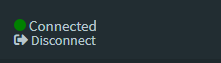
• Functions to manage the “Connected” / “No connection” display. It’s a bunch of logic and CSS to just control a small element of the GUI. Basically if the variable connection$active is TRUE the GUI will show “Connected” next to a green dot with a “Disconnect” button, otherwise it will display “No connection” next to a red dot. When the button “Disconnect” is pressed, the function to log out of the server is triggered and the connection$active variable is set to false.
• Stop function: This delcaration is left for future developers. When having trouble on a certain spot, add a stop button using actionButton("stop", "stop"), press it on the GUI to stop the execution and perform the required debugging.

The scripts sourced for by the server.R are the following:

4.1.2.1 connection.R

This is probably the most important script of the whole application, as it’s the one that is responsible for loading the data in order to ensure that the application capabilities can be extended in the future painlessly (modular).

Inside this script there are five different sections that are triggered by different actions:

1. Creation of GUI for the new server tabs
2. Creation of observeEvents for all the different server tab elements.
   1. URL builder to display selected items on a browser
   2. Connection to the server to obtain the projects and resources. Triggered by the button with label “connect_server.”
   3. Get tables / resources from the selected project. Triggered everytime the selector with label “project_selected” is changed.
   4. Add a study. Triggered by the button with label “add_server.”
3. Remove a server tab. Triggered by the button with label “remove.”
4. Remove a study item Triggered by the button with label “remove_item.”
5. Load the selected studies to the study servers. Triggered by the button with label “connect_selected.”

The first element to explain is the creation of the new server tabs (Point 1, observeEvent(input$add, {})). It’s just a matter of noting two things to understand it easily, 1) The use of a reactive value tabIndex() which returns a integer (initialized at 1), this integer corresponds to the tab being created (hence it’s updated at the top of the call); 2) The rest of the call is an appendTab() that adds a new tab on the element id "tabset1" with the exact structure of ui.R but changing the element IDs using the reactive value so that all the buttons/input fields are numbered according to the tab they are located on. When removing a server tab (observeEvent(input$remove, {})) the tab itself is removed using removeTab() and the reactive value is actualized.

The creation of observeEvents for all the different server tab elements (Subitems of point 2) is done using a small trick. max_servers number of observeEvents are created (using lapply) for the different functionalities so that all the server tabs are functional, this integer variable is defined on the script server.R, if more servers than the default (10) are required just update the definition of the variable and relaunch the application.

The last part of the script, loads all the selected tables and resources to the selected study servers. It does everything needed to each particular type of resource, that means converting them to R objects or to tables depending on what they are.

When loading the selected resources or tables into the study servers, the table available_tables is created. The name is a little bit confusing since it actually contains the information about tables and resources, the developer apologizes as this variable was set at the beginning of the development and has not been updated. Nevertheless, it’s an important variable of the application, the structure of this table is the following.

Column	Description
name	Name of the object (project.name)
server_index	Index of the study server that contains the table/resource
server	Name of the study server
type_resource	Type of the resource

The Opal server can host different types of resources, to name a few there are ExpressionSet, RangedSummarizedExperiment and SQLResourceClient. Each type of resource needs a special treatment to be used, for example SQLResourceClient resources are plain tables, so they need to be converted to tables on the study server to use them. Currently the following resource types are supported by ShinyDataSHIELD.

Resource type	Treatment	Name of the resource type on available_tables
TidyFileResourceClient, SQLResourceClient	- as.resource.data.frame(resource) - Append .t to the name	table
SshResourceClient	Append .r to the name	ssh
GdsGenotypeReader	- as.resource.object(resource) - Append .r to the name	r_obj_vcf
ExpressionSet	- as.resource.object(resource) - Append .r to the name	r_obj_eset
RangedSummarizedExperiment	- as.resource.object(resource) - Append .r to the name	r_obj_rse
Any other resource type	- as.resource.object(resource) - Append .r to the name	r_obj

.r and .t are appended to the resources to allow a resource and a table on the same project to have the same names and not crash the Shiny application.

Now, let’s look at some examples to add new resource types on the connection.R file. There are different cases for the treatment that the new resource requires.

• Resources that just need to be loaded with no further action performed to them (same treatment as SSH connections). Add another else if statement after line 303. Example: New resource called Simple_resource

else if ("Simple_resource" %in% resource_type){
            # Update available_tables list with the new resource type name
lists$available_tables <- rbind(lists$available_tables, c(name = name, server_index = server_index,
                                                                      server = resources$study_server[i], type_resource = "Simple_resource"))
          }

• Resources that need to be converted into R objects (datashield.assign.expr(conns, symbol = "methy", expr = quote(as.resource.object(res)))) and nothing else. Will work out of the box (the type_resource column of the lists$available_tables table will read r_obj).
• Resources that need to be converted into R objects (datashield.assign.expr(conns, symbol = "methy", expr = quote(as.resource.object(res)))) and be further processed. Add another else if statement after line 320. Example: A new type of resource called special_resource that contains some variable names that are desired to be saved on a variable to feed a list on the GUI.

else if("special_resource" %in% resource_type) {
              # Update available_tables list with the new resource type name
  lists$available_tables <- rbind(lists$available_tables, c(name = name, server_index = server_index,
                                                                        server = resources$study_server[i], type_resource = "special_resource"))
              # Perform the needed actions for this resource
              [...]
            }

Finally, once all the connections have been successful, and all the selected tables and resources are loaded, the tabs that make use of the loaded objects are enabled by using (table examples)

if(any(unique(lists$available_tables$type_resource) %in% c("table"))) {
        show(selector = "ul li:eq(2)")
      }

There are many if that checks for type of resources and enables tabs if present, on the previous example the second tab ul li:eq(2) (there is no way of refering them by ID as far as I know to perform this action) is enabled because it contains a module that works with tables.

If a new type of resource is implemented, add after line 353 (tab 10 is just as example)

if(any(unique(lists$available_tables$type_resource) %in% c("new_resource"))) {
        show(selector = "ul li:eq(10)")
      }

Also update this part if a new module is added, make sure to enable the tab only when the resources that the module use are present on the lists$available_tables.

4.1.3 Structure of the modules

A common structure is followed for all the different modules, this refers to the general structure of descriptive_stats.R, statistics_models.R, genomics.R, omics.R and table_columns.R.

Before describing the internal structure of the modules, let’s briefly describe the GUI structure, which is also common between them. The tabs are filled with a tab box, the first element is always a table with the available tables / resources for that module. For example, the Omics module only displays the resources of type RSE or eSet. The other tabs are disabled by default and can only be accessed once the user has selected which resource to use. Now let’s talk about how to accomplish all of this.

At the beginning of all the modules there is an observeEvent that is triggered when the user selects an item from the table. The structure of this is the following

observeEvent(input$table, {
  if(length(input$table_rows_selected) > 0){ # Check if the user has selected any row
    different_study_server <- TRUE # On this example we are checking that everything selected is on different study servers
    same_cols <- TRUE # On this example we are checking tables to be pooled, so we are checking they have the same columns
    if(length(input$table_rows_selected) > 1){ # If more than one table is selected the checks have to be performed, otherwise there is no need to check for same cols or different study servers
      same_cols <- all(lapply(input$tqble_rows_selected, function(i){
        res<-all(match(lists$resource_variables[[as.character(lists$available_tables[type_resource %in% c("table")][i,1])]], 
                       lists$resource_variables[[as.character(lists$available_tables[type_resource %in% c("table")][1,1])]]))
        if(is.na(res)){FALSE} else{res}
      }))
      different_study_server <- nrow(unique(lists$available_tables[input$table_rows_selected,3])) ==
        length(input$table_rows_selected) 
    }
    if(same_cols & different_study_server){ # If both tests are OK, remove the "resource_lim" object from the study servers
      datashield.rm(connection$conns, "resource_lim")
      for(i in input$table_rows_selected){
        lists$available_tables[type_resource %in% c("table")][i,2]
        # Then assign the selected tables to a new variable on the study servers called "resource_lim", this is the variable that all the other funcionalities of the module will refer to when performing analysis
        datashield.assign.expr(connection$conns[as.numeric(lists$available_tables[type_resource %in% c("table")][i,2])], "resource_lim", as.symbol(as.character(lists$available_tables[type_resource %in% c("table")][i,1])))
      }
      # Enable the analysis tab and update the GUI to display it
      js$enableTab("tab_of_analysis")
      updateTabsetPanel(session, "id",
                        selected = "tab_of_analysis")
    }
    else{ # If the tests fail, display an error message
      shinyalert("Oops!", 
                 if(!same_cols){
                   "Selected resources do not share the same columns, can't pool unequal resources"
                 }else{
                   "Selected resources are not on different study servers, can't pool resources on the same study server."
                 }
                 , type = "error")
      # Make sure analysis tabs are disabled and the GUI shows the selection tab, this is important to do because if the user first selects a valid table and then an invalid combination, we want to make sure that the user has no longer access to the analysis tab
      js$disableTab("tab_of_analysis")
      updateTabsetPanel(session, "id",
                        selected = "table_selection")
    }
  }
})

This example can be extended to the developers needs, but as a structure example is more than enough. Please read the source code for the available modules if extra examples are needed.

The body of the modules correspond to whatever is needed on that module, let that be some observeEvent for buttons of the analysis tab, some renderUI for dynamic selectors or anything other that the module needs.

The bottom of the modules is also shared, they contain an observe clause that is triggered when the tab is selected, it has the following structure

observe({
  if(input$tabs == "id") { # The ID here corresponds to the tabname declare on the ui.R ; tabItem(tabName = "ID", ....... 
    tables_available <- lists$available_tables[type_resource %in% c("table")] # Input here the type_resource that this module uses, so only those are displayed
    if(length(lists$resource_variables) == 0){
      withProgress(message = "Reading column names from available tables", value = 0, {
        for(i in 1:nrow(tables_available)){ # In this example we are reading table columns so that when the user selects from this table, we can automatically check if the columns are shared when trying to pool tables, this is done on the header of the module, that we have just seen
          lists$table_columns[[as.character(tables_available[i,1])]] <- ds.colnames(as.character(tables_available[i,1]), datasources = connection$conns[as.numeric(tables_available[i,2])])[[1]]
          incProgress(i/nrow(tables_available))
        }
      })
    }
    # Finally we render the table with the available tables for this module so the user can select which ones to use, of course this needs to be completed on the table_renders.R (following chunk has an example)
    output$available_tables_sm <- renderUI({
      dataTableOutput("available_tables")
    })
  }
})

Example of the code for the table_render.R regarding the selection table

output$available_tables <- renderDT(
  lists$available_tables[type_resource == "table"], options=list(columnDefs = list(list(visible=FALSE, targets=c(0,2,4))),
                                                                 paging = FALSE, searching = FALSE)
)

Now let’s take a look at the scripts that are used by all the modules, their use is to render tables, figures and handle the downloads (figures + table downloads)

4.1.3.1 table_renders.R

This script creates the displays of all the tables of ShinyDataSHIELD, it uses the DT package to do so. Besides the descriptive_summary table, all the other tables just render results from other functions.

There are some things to point of this script:

• As can be seen in descriptive_summary table, you can actually perform operations inside of a renderDT function and display the result of them.
• The most used options for the tables aesthetics are the following

options=list(columnDefs = list(list(visible=FALSE, targets=c(0))),
                                          paging = FALSE, searching = FALSE)

This prevents the rownames column to be displayed (usually it just contains the numeration of rows 1…N, be aware sometimes it’s of interest to see this column) and eliminates the paging and searching functionalities of the table. For small tables it makes sense to not show that but on big tables those options are set to TRUE, as it’s very useful to have a search box on them.

• The tables that display numerical columns (mixed or not with non-numerical columns) are actually passed through the format_num function (defined on server.R) so the displayed table has only four decimals but the actual table (the one that can be saved) has all the decimals. This is done using the following code

as.data.table(lapply(as.data.table(vcf_results$result_table_gwas$server1), format_num))

This will pass each column to the function and if it’s numerical the decimals will be cut to 4.

• The table output structure of the LIMMA results look different than the others, this is because when performing a LIMMA with pooled resources it returns one table for each study, what is being done is just binding them to display to the user all the obtained results.

There is a concrete render that needs a special mention on this documentation, that is the column_types_table, which uses the CellEdit JavaScript plugin to enable drop down menus when editing a table. Let’s see what is being done

tab <- datatable(
      table_to_be_modified, editable = "cell", callback =  # The callback needs to be updated to include the JS custom code
        JS(
          "function onUpdate(updatedCell, updatedRow, oldValue){",
          "Shiny.onInputChange('jsValue', [updatedCell.index(), updatedCell.data()]);", # The results to actually update the table_to_be_modified on the module script will be retrieved by a observeEvent(input$jsValue, { ; change jsValue each time this approach is used to avoid collisions
          "}",
          "table.MakeCellsEditable({",
          "  onUpdate: onUpdate,",
          "  inputCss: 'my-input-class',",
          "  columns: [2],",
          "  confirmationButton: {",
          "    confirmCss: 'my-confirm-class',",
          "    cancelCss: 'my-cancel-class'",
          "  },",
          "  inputTypes: [",
          "    {",
          "      column: 2,",
          "      type: 'list',",
          "      options: [",
          "        {value: 'numeric', display: 'numeric'},", # Update this lines to declare the options of the dropdown
          "        {value: 'factor',      display: 'factor'},",
          "        {value: 'character',    display: 'character'}",
          "      ]",
          "    }",
          "  ]",
          "});"),
      options = list(pageLength = nrow(table_to_be_modified))
    )
    path <- "../../www/" # folder containing the files dataTables.cellEdit.js
    # and dataTables.cellEdit.css, they are already included on ShinyDataSHIELD, so there is no need to worry about that
    dep <- htmltools::htmlDependency(
      "CellEdit", "1.0.19", path,
      script = "dataTables.cellEdit.js", stylesheet = "dataTables.cellEdit.css")
    tab$dependencies <- c(tab$dependencies, list(dep))

Example of what to include on the module script to update the table

proxy = dataTableProxy('a') # No need to change this
observeEvent(input$jsValue, { # As stated above, the trigger is actually the value defined on the callback, we can retrieve the row, column and value from that object
  change <- data.table(input$jsValue)
  row <- as.numeric(change[1,1]) + 1
  column <- as.numeric(change[2,1])
  value <- as.character(change[4,1])
  
  table_to_be_modified[row, column] <<- value
  replaceData(proxy, table_to_be_modified, resetPaging = FALSE)
}

4.1.3.2 plot_renders.R

There are two types of plots on ShinyDataSHIELD, the ones created with the base function plot and the ones created with the ggplot library. In order to later recover the plots to download them, they actually have a different structure.

• Base plot structure:

output$random_plot <- renderPlot({
  plots$random_plot <- function(){
    function_that_generates_the_plot_using_base_package(arguments)
  }
  plots$random_plot()
})

For the base plots, a function is declared that returns the plot and is called to generate the plot to the GUI.

• Ggplot structure:

output$manhattan <- renderPlot({
  plots$ggplot <- function_that_generates_the_plot_using_ggplot2_package(arguments)
  plots$ggplot
})

In this case the plot is saved, ggplot will generate a plot variable that can be called to render the plot.

On this script there are two plots that are inside a renderCachedPlot function instead of a renderPlot because they take really long to calculate and it’s better to cache them.

Inside of the renderPlot function some other code can be put, such as toggles to GUI elements or tryCatch() functions.

4.1.3.3 download_handlers.R

In this script everything related to downloading plots and tables is found. There are basically three types of structures

• Table downloader: To download a *csv. Structure:

output$table_download <- downloadHandler(
  filename = "table.csv",
  content = function(file) {
    write.csv(
      variable_that_contains_table
      , file, row.names = FALSE)
  }
)

The row.names = FALSE argument may not be needed in tables where the row names are important.

• Base plot downloader: To download a *.png. Structure:

output$base_plot_download <- downloadHandler(
  filename = "base_plot.png",
  content = function(file) {
    png(file = file)
    plots$base_plot()
    dev.off()
  }
)

Basically this calls the previously declared function and captures the plot into a *.png.

• GGplot downloader: To download a *.png. Structure:

output$ggplot_download <- downloadHandler(
  filename = "ggplot.png",
  content = function(file) {
    ggsave(file, plot = last_plot())
  }
)

When using ggplot, the function last_plot() renders the last plot rendered by ggplot. This only has one inconvenient, that is when you are downloading a plot that takes a while to render, the application doesn’t show the save window dialog until it has rendered again. This should be addressed in the future as it really halters the user experience.

4.1.4 How to add a new block

To add a new block to ShinyDataSHIELD, the developer has to create a new *.R script inside the inst/shinyApp/ folder of the project and give it a descriprive name of the function that it will perform.

So the Shiny application actually sees it, the server.R needs to be updated and source the new file. Example: New block called new_analysis.R, the update to the server.R will be

source("new_analysis.R", local = TRUE)

Afterwards, the ui.R can be updated by defining how the new block will be presented to the user. The sidebarMenu function needs to be updated so that the new tab appears on the sidebar of the application, follow the structure of the other tabs. Afterwards update the dashboardBody function by defining all the different elements of the new tab, follow the structure of the other available tabs to follow the general design lines, all the functions that need to be used here are standard Shiny functions mostly and there’s plenty of documentation and examples available online, when in doubt just try to copy an already implemented structure.

Now the user can focus on the types of files that will feed this new block, if it’s a table there’s no need to worry, if it’s a resource that is not implemented the connection.R needs to be updated. Read the above documentation for guidance on the changes that need to be done for new resources types.

Once the GUI is setup and the table / resource that this block will use is setup, the backend for this block can be built on the new_analysis.R file. Include on that file all the required renderUI() functions and steps to process the file and analyze it. Probably a new variable will be required to hold the results, update the server.R header and include a new reactiveValues() declaration for the new block.

If the new block requires to display tables or figures, update the table_renders.R and plot_renders.R following the given examples on their sections of the documentation. Make sure to include the download buttons for them on the download_handlers.R.

If there is some part of the code that takes some time to process, there’s the option of wrapping it inside the withProgress() function in order to display a loading annimation to the GUI to alert the user that something is being processed.

Make sure to include the custom implementation of the header and footer functions for the module that have been presented before.

When developing a new block there will probably be many problems occurring, in order to debug a Shiny application there is the browser() function, if the developer is getting some sort of error at X line of the script, just write browser() on the line adobe of the error, the execution will be stopped at that point and the developer can interact with all the available variables of the environment through the RStudio console, usually running the line that is giving an error on the console will provide enough information to kill the bug. If the line breaking is a function call it is advisable to type the variables that are being passed into the function on the console, that way the developer can see what exactly is being passed and can see that some argument is NULL when it shouldn’t or it’s a character when it should be a number, those are quite common problems.

When a new block is developed and integrated into ShinyDataSHIELD, please conclude it by updating this documentation and the user guide with a brief explanation of the new block and some remarks of the most interesting bits of it.