General demonstration • dsOMOPHelper

This demonstration showcases the use of the dsOMOPHelper package, which provides a simplified approach for extracting data from OMOP CDM databases and integrating it with the DataSHIELD workflow through the dsOMOPClient package. dsOMOPHelper allows for the extraction and use of data from an OMOP CDM database as needed, based on the variables chosen by the user, formatting the data to make the information more accessible to researchers from the DataSHIELD environment. To assist in selecting data from the database, the package also includes methods for exploring the data that is available in the database.

It is important to note that dsOMOPHelper aims to show the enhanced capabilities of tools built on top of dsOMOPClient by making its operations simpler and automating many of its processes. However, this ease of use might limit options for edge case situations that demand very specific operations, where using the basic methods of dsOMOPClient might be more appropriate due to its flexibility. For further technical information about the dsOMOPClient package, or if you’re considering developing a tool based on it for a particular goal, please refer to its GitHub repository.

Prerequisites

Before using dsOMOPHelper, it is recommended to have a basic understanding of:

The OMOP CDM structure and its standardized clinical data format. You can learn more about OMOP CDM in the OHDSI Book chapter ‘The Common Data Model’.
OMOP Vocabularies and how they standardize medical concepts (like diagnoses, medications, procedures) across different coding systems (ICD-9, ICD-10, SNOMED CT, etc.) into a common representation. The OHDSI Book chapter ‘Standardized Vocabularies’ provides a comprehensive overview of this standardization process.
Basic DataSHIELD concepts and workflow. The DataSHIELD Beginner’s Tutorial is a good starting point.

This knowledge will help you better understand how to effectively query and work with OMOP CDM data through the DataSHIELD infrastructure.

Establishing a connection

In this example, we will be using the MIMIC IV data available on the OBiBa’s public Opal demo server. This server is publicly accessible, so all users are able to reproduce the examples of this guide by executing the same commands in their R session. The access credentials are:

Server URL: https://opal-demo.obiba.org
User: dsuser
Password: P@ssw0rd
Profile: omop

First, we will establish a connection to the demo server using DSI with the provided credentials:

library(DSI)
library(DSOpal)
library(dsBaseClient)
library(dsOMOPClient)
library(dsOMOPHelper)

builder <- newDSLoginBuilder()
builder$append(
  server = "opal_demo",
  url = "https://opal-demo.obiba.org",
  user = "dsuser",
  password = "P@ssw0rd",
  profile = "omop"
)
logindata <- builder$build()
conns <- datashield.login(logins = logindata)

Creating an interface helper object

Once we have successfully established a connection with the server, we will create an interface helper object with ds.omop.helper. This function creates an interface object that allows users to interact with the OMOP CDM database based on a resource. We can use the methods available in this object to obtain data from the database by applying the desired filters and querying data catalogs for information present in the database.

Our server contains the database connection resource under the name mimiciv within the omop_demo project. Therefore, we need to specify that, from the connection we have established, we want to take the omop_demo.mimiciv resource. We also need to specify the symbol we want to use to refer to this object. In this case, we will use mimiciv as the symbol name:

o <- ds.omop.helper(connections = conns,
                    resource = "omop_demo.mimiciv",
                    symbol = "mimiciv")

When creating the helper object, the data from the Person table is automatically loaded into the specified symbol, in this case, mimiciv. We can check the contents of this symbol by using the ds.summary function from dsBaseClient:

ds.summary("mimiciv")

## $opal_demo
## $opal_demo$class
## [1] "data.frame"
## 
## $opal_demo$`number of rows`
## [1] 100
## 
## $opal_demo$`number of columns`
## [1] 5
## 
## $opal_demo$`variables held`
## [1] "person_id"            "gender_concept_id"    "year_of_birth"       
## [4] "race_concept_id"      "ethnicity_concept_id"

Therefore, we will be using the Person table as the foundation since it serves as a central link to other clinical data tables in OMOP CDM databases. From here, we will build our study-specific table by adding the necessary data from other tables based on the variables required for our particular study.

Exploring the data

Before we can construct our own study table, it’s essential that we understand what data is available in the database. To achieve this, we can use the data exploration methods provided by ds.omop.helper, which allow us to identify the available tables in the database, as well as the concepts and columns that each table contains.

Tables

The tables method returns a list of the available tables in the database:

o$tables()

## $opal_demo
##  [1] "attribute_definition" "care_site"            "cdm_source"          
##  [4] "cohort"               "cohort_attribute"     "cohort_definition"   
##  [7] "concept"              "concept_relationship" "condition_era"       
## [10] "condition_occurrence" "cost"                 "death"               
## [13] "device_exposure"      "dose_era"             "drug_era"            
## [16] "drug_exposure"        "fact_relationship"    "location"            
## [19] "measurement"          "metadata"             "note"                
## [22] "note_nlp"             "observation"          "observation_period"  
## [25] "payer_plan_period"    "person"               "procedure_occurrence"
## [28] "provider"             "specimen"             "visit_detail"        
## [31] "visit_occurrence"     "vocabulary"

Concepts

The concepts method returns a data frame that functions as a dictionary for the available concepts within a specific table. Here, concept_id refers to the identifier of the present concepts, and concept_name is the textual name assigned to each concept.

For instance, if we want to explore the concepts available in the Condition_occurrence table:

o$concepts("condition_occurrence")

## $opal_demo
##    concept_id             concept_name
## 1       27674      Nausea and vomiting
## 2       29735     Candidiasis of mouth
## 3       31317                Dysphagia
## 4       73553              Arthropathy
## 5       75576 Irritable bowel syndrome
## 6       75860             Constipation
## 7       77670               Chest pain
## 8       78232      Shoulder joint pain
## 9       79864       Hematuria syndrome
## 10      80180           Osteoarthritis
##  [ reached 'max' / getOption("max.print") -- omitted 236 rows ]

Columns

The columns method returns a list of the available column names in a specific table. This enables us to understand what information we can extract from each table, allowing us to select only the columns necessary for our study:

o$columns("condition_occurrence")

## $opal_demo
## $opal_demo$condition_occurrence
##  [1] "condition_occurrence_id"       "person_id"                    
##  [3] "condition_concept_id"          "condition_start_date"         
##  [5] "condition_start_datetime"      "condition_end_date"           
##  [7] "condition_end_datetime"        "condition_type_concept_id"    
##  [9] "stop_reason"                   "provider_id"                  
## [11] "visit_occurrence_id"           "visit_detail_id"              
## [13] "condition_source_value"        "condition_source_concept_id"  
## [15] "condition_status_source_value" "condition_status_concept_id"

Retrieving tables

Having explored the data available in the database, we are now ready to build our study-specific table. To do this, we’ll employ the auto method provided by dsOMOPHelper. This method simplifies the task by automatically extracting and appending variables from various tables to our initial table (which currently only includes data from the Person table).

The auto method uses the following arguments:

tables: A character vector of the names of the tables from which we want to extract data.
concepts: A numeric vector of the concept IDs of the concepts we want to extract.
columns: A character vector of the column names in the tables from which we want to extract data.

All of these are optional, but it is highly recommended to utilize them to expedite the data extraction process and the construction of the study table.

For instance, let’s assume that, after the data exploration phase using the methods described above, we have decided to extract data on the condition Cardiac arrhythmia, which has a concept ID of 44784217 and is found in the Condition_occurrence table, and the observation Body mass index 40+ - severely obese, with a concept ID of 4256640 located in the Observation table. We want all columns related to both variables, so we will not specify any column filters.

Our call to the auto method would be as follows:

o$auto(tables = c("condition_occurrence", "observation"),
       concepts = c(44784217, 4256640))

ds.summary("mimiciv")

## $opal_demo
## $opal_demo$class
## [1] "data.frame"
## 
## $opal_demo$`number of rows`
## [1] 100
## 
## $opal_demo$`number of columns`
## [1] 18
## 
## $opal_demo$`variables held`
##  [1] "person_id"                                                    
##  [2] "gender_concept_id"                                            
##  [3] "year_of_birth"                                                
##  [4] "race_concept_id"                                              
##  [5] "ethnicity_concept_id"                                         
##  [6] "cardiac_arrhythmia.condition_occurrence_id"                   
##  [7] "cardiac_arrhythmia.condition_start_date"                      
##  [8] "cardiac_arrhythmia.condition_start_datetime"                  
##  [9] "cardiac_arrhythmia.condition_end_date"                        
## [10] "cardiac_arrhythmia.condition_end_datetime"                    
## [11] "cardiac_arrhythmia.condition_type_concept_id"                 
## [12] "cardiac_arrhythmia.visit_occurrence_id"                       
## [13] "body_mass_index_40_severely_obese.observation_id"             
## [14] "body_mass_index_40_severely_obese.observation_date"           
## [15] "body_mass_index_40_severely_obese.observation_datetime"       
## [16] "body_mass_index_40_severely_obese.observation_type_concept_id"
## [17] "body_mass_index_40_severely_obese.value_as_string"            
## [18] "body_mass_index_40_severely_obese.visit_occurrence_id"

As we can see, the table mimiciv now contains information from the Condition_occurrence and Observation tables, with all the columns related to our variables of interest.

Examples of usage

In this section, we will explore some examples of how we can use the data extraction functions of dsOMOPHelper in conjunction with DataSHIELD’s environment functions to manipulate and analyze the data.

Let’s say that we want to add the observation Marital status [NHANES] to our study table. To do this, we first need to identify the corresponding concept, which in this case is 40766231 and is found in the Observation table of the database. In this instance, since we are only interested in its primary value and it is a categorical variable, we aim to retrieve data from the value_as_concept_id column.

Our call to the auto function would be as follows:

o$auto(tables = c("observation"),
       concepts = c(40766231),
       columns = c("value_as_concept_id"))

ds.summary("mimiciv$marital_status_nhanes.value_as_concept_id")

## $opal_demo
## $opal_demo$class
## [1] "factor"
## 
## $opal_demo$length
## [1] 100
## 
## $opal_demo$categories
## [1] "divorced"      "married"       "never_married" "widowed"      
## 
## $opal_demo$`count of 'divorced'`
## [1] 10
## 
## $opal_demo$`count of 'married'`
## [1] 36
## 
## $opal_demo$`count of 'never_married'`
## [1] 30
## 
## $opal_demo$`count of 'widowed'`
## [1] 12

As we can see, we have successfully obtained a categorical variable containing the marital status information of the patients, specifically with the following categories: divorced, married, never_married, widowed. Now, we can use the ds.table function from dsBaseClient to obtain a frequency table of that same variable:

ds.table("mimiciv$marital_status_nhanes.value_as_concept_id")

## 
##  Data in all studies were valid 
## 
## Study 1 :  No errors reported from this study

## $output.list
## $output.list$TABLE_rvar.by.study_row.props
##                                                  study
## mimiciv$marital_status_nhanes.value_as_concept_id opal_demo
##                                     divorced              1
##                                     married               1
##                                     never_married         1
##                                     widowed               1
##                                     NA                    1
## 
## $output.list$TABLE_rvar.by.study_col.props
##                                                  study
## mimiciv$marital_status_nhanes.value_as_concept_id opal_demo
##                                     divorced           0.10
##                                     married            0.36
##                                     never_married      0.30
##                                     widowed            0.12
##                                     NA                 0.12
## 
## $output.list$TABLE_rvar.by.study_counts
##                                                  study
## mimiciv$marital_status_nhanes.value_as_concept_id opal_demo
##                                     divorced             10
##                                     married              36
##                                     never_married        30
##                                     widowed              12
##                                     NA                   12
## 
## $output.list$TABLES.COMBINED_all.sources_proportions
## mimiciv$marital_status_nhanes.value_as_concept_id
##      divorced       married never_married       widowed            NA 
##          0.10          0.36          0.30          0.12          0.12 
## 
## $output.list$TABLES.COMBINED_all.sources_counts
## mimiciv$marital_status_nhanes.value_as_concept_id
##      divorced       married never_married       widowed            NA 
##            10            36            30            12            12 
## 
## 
## $validity.message
## [1] "Data in all studies were valid"

We now want to extract a numerical variable, for instance, Body weight, which is identified by the concept ID 3025315 and is located in the Measurement table. In this scenario, our goal is to retrieve data from the value_as_number column.

Our call to the auto function would be as follows:

o$auto(tables = c("measurement"),
       concepts = c(3025315),
       columns = c("value_as_number"))

ds.summary("mimiciv$body_weight.value_as_number")

## $opal_demo
## $opal_demo$class
## [1] "numeric"
## 
## $opal_demo$length
## [1] 100
## 
## $opal_demo$`quantiles & mean`
##        5%       10%       25%       50%       75%       90%       95% 
##  52.43500  59.26000  68.70000  80.00000  97.22500 121.95000 149.09000 
##      Mean 
##  86.80918

As we can see, we have successfully obtained a numerical variable that contains the body weight of the patients. To visually inspect the distribution of that same variable, we can generate a histogram using the ds.histogram function from dsBaseClient:

ds.histogram("mimiciv$body_weight.value_as_number")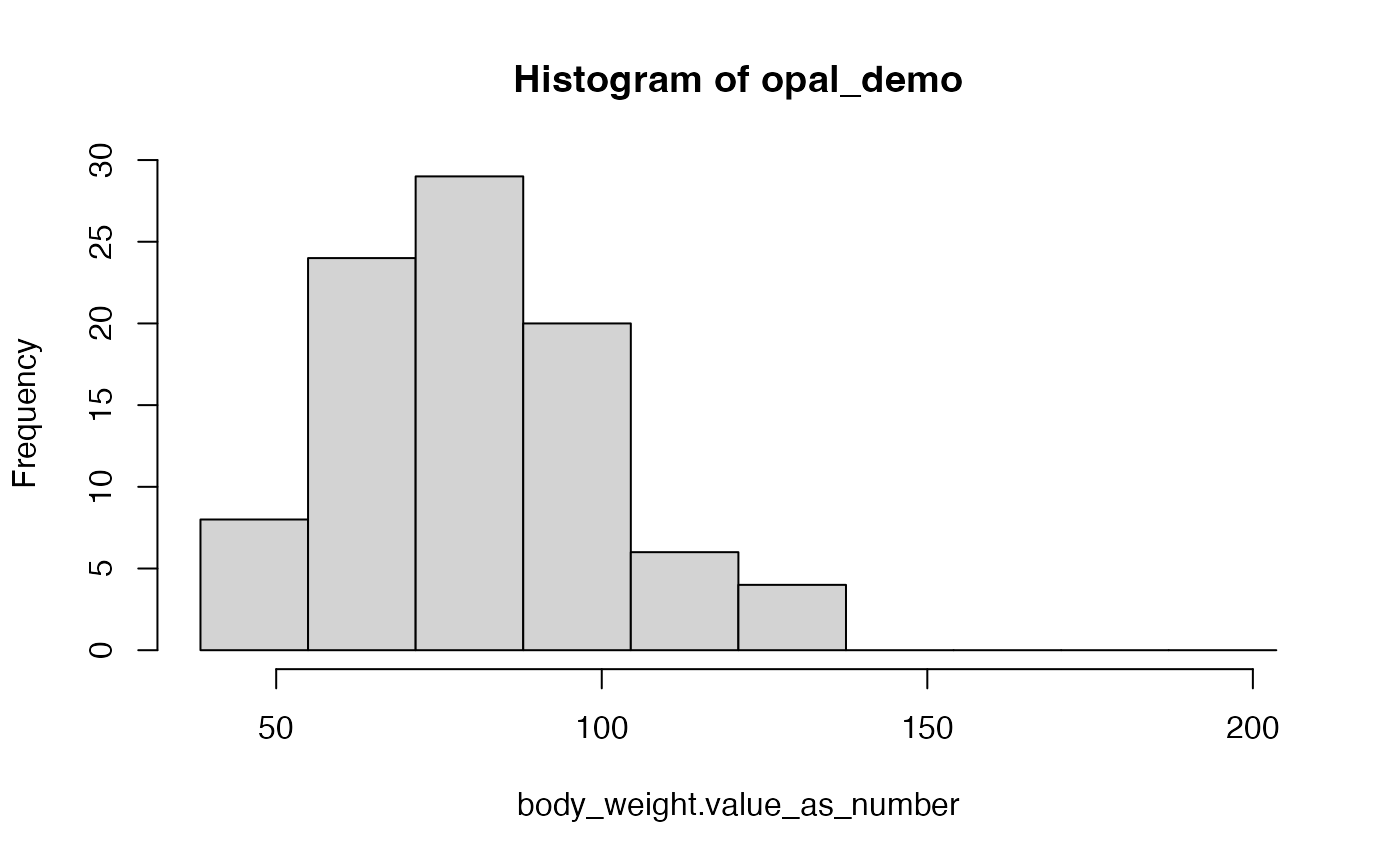

## $breaks
##  [1]  38.37067  54.89376  71.41685  87.93995 104.46304 120.98613 137.50922
##  [8] 154.03231 170.55540 187.07849 203.60158
## 
## $counts
##  [1]  8 24 29 20  6  4  0  0  0  0
## 
## $density
##  [1] 0.004940519 0.014821558 0.017909383 0.012351299 0.003705390
##  [6] 0.002470260 0.000000000 0.000000000 0.000000000 0.000000000
## 
## $mids
##  [1]  46.63222  63.15531  79.67840  96.20149 112.72458 129.24767 145.77076
##  [8] 162.29386 178.81695 195.34004
## 
## $xname
## [1] "xvect"
## 
## $equidist
## [1] TRUE
## 
## attr(,"class")
## [1] "histogram"

Finally, we will perform a generalized linear regression (GLM) analysis to evaluate the relationship between blood glucose, hemoglobin A1c, and vitamin B12. To do this, we first need to extract the variables of interest from the corresponding tables, which are present in the Measurement table.

For blood glucose, we use the concept ID 3000483, which corresponds to Glucose [Mass/volume] in Blood. For hemoglobin A1c, the concept ID is 3004410, representing Hemoglobin A1c/Hemoglobin.total in Blood. Lastly, for vitamin B12, we refer to the concept ID 3000593, linked to Cobalamin (Vitamin B12) [Mass/volume] in Serum or Plasma. Our objective is to extract the numerical values for these variables, hence we will focus on retrieving data specifically from the value_as_number column.

Once the data is extracted, we can use the ds.glm function from dsBaseClient to perform the generalized linear regression analysis:

o$auto(tables = c("measurement"),
       concepts = c(3000483, 3004410, 3000593),
       columns = c("value_as_number"))

ds.glm(formula = "glucose_mass_volume_in_blood.value_as_number ~ 
                  hemoglobin_a1c_hemoglobin_total_in_blood.value_as_number + 
                  cobalamin_vitamin_b12_mass_volume_in_serum_or_plasma.value_as_number",
       data = "mimiciv",
       family = "gaussian",
       datasources = conns)

## $Nvalid
## [1] 10
## 
## $Nmissing
## [1] 90
## 
## $Ntotal
## [1] 100
## 
## $disclosure.risk
##           RISK OF DISCLOSURE
## opal_demo                  0
## 
## $errorMessage
##           ERROR MESSAGES
## opal_demo "No errors"   
## 
## $nsubs
## [1] 10
## 
## $iter
## [1] 3
## 
## $family
## 
## Family: gaussian 
## Link function: identity 
## 
## 
## $formula
## [1] "glucose_mass_volume_in_blood.value_as_number ~ hemoglobin_a1c_hemoglobin_total_in_blood.value_as_number +      cobalamin_vitamin_b12_mass_volume_in_serum_or_plasma.value_as_number"
## 
## $coefficients
##                                                                          Estimate
## (Intercept)                                                          112.32082034
## hemoglobin_a1c_hemoglobin_total_in_blood.value_as_number               2.02330303
## cobalamin_vitamin_b12_mass_volume_in_serum_or_plasma.value_as_number  -0.01508464
##                                                                       Std. Error
## (Intercept)                                                          87.86777856
## hemoglobin_a1c_hemoglobin_total_in_blood.value_as_number             11.23987059
## cobalamin_vitamin_b12_mass_volume_in_serum_or_plasma.value_as_number  0.04190505
##                                                                         z-value
## (Intercept)                                                           1.2782936
## hemoglobin_a1c_hemoglobin_total_in_blood.value_as_number              0.1800112
## cobalamin_vitamin_b12_mass_volume_in_serum_or_plasma.value_as_number -0.3599719
##                                                                        p-value
## (Intercept)                                                          0.2011459
## hemoglobin_a1c_hemoglobin_total_in_blood.value_as_number             0.8571437
## cobalamin_vitamin_b12_mass_volume_in_serum_or_plasma.value_as_number 0.7188681
##                                                                         low0.95CI
## (Intercept)                                                          -59.89686103
## hemoglobin_a1c_hemoglobin_total_in_blood.value_as_number             -20.00643853
## cobalamin_vitamin_b12_mass_volume_in_serum_or_plasma.value_as_number  -0.09721702
##                                                                        high0.95CI
## (Intercept)                                                          284.53850171
## hemoglobin_a1c_hemoglobin_total_in_blood.value_as_number              24.05304458
## cobalamin_vitamin_b12_mass_volume_in_serum_or_plasma.value_as_number   0.06704774
## 
## $dev
## [1] 20986.45
## 
## $df
## [1] 7
## 
## $output.information
## [1] "SEE TOP OF OUTPUT FOR INFORMATION ON MISSING DATA AND ERROR MESSAGES"

As we can see, the data extracted from dsOMOPHelper can be perfectly integrated with DataSHIELD’s environment functions to perform a wide range of operations, from simple descriptive statistics to more complex statistical modeling.

However, due to the reduced size of the sample data available in the public demo server, the results of the GLM analysis are not statistically significant. For a statistically significant analysis, we have included a COPD analysis vignette that reproduces some studies from the literature using a larger database that is not publicly available in the demo server.

Logout

After finishing the analysis, it is important to logout from the DataSHIELD server to free up resources:

datashield.logout(conns)