COPD analysis example
copd.RmdIntroduction
In this analysis, we explore the relationship between chronic
obstructive pulmonary disease (COPD) and several key predictors using a
synthetic dataset. Our goal is to demonstrate how dsOMOP
can be used to analyze clinical data while validating known clinical
associations.
We utilize the Tufts Synthetic Dataset, which consists of fully synthetic electronic health record (EHR) data representing 567,000 synthetic patients. This dataset was generated in 2021 through a collaboration between Syntegra, Inc. and Tufts Medical Center using a deep learning transformer model. The model was trained on real-world EHR data from the Tufts Research Data Warehouse (TRDW), which had already been transformed into OMOP CDM format. It includes longitudinal clinical data from patients who received care across Tufts Medicine’s three hospitals, 40-practice physician network, and home health care organization.
The Tufts Synthetic Dataset contains clinical information such as patient visits, conditions, medications, laboratory measurements, procedures, observations, and device exposures, all structured according to the OMOP CDM version 5.3. The large volume of patient data, along with the realistic nature of the synthetic dataset, makes it ideal for testing the functionality of dsOMOP by exploring significant associations and patterns within the data.
Based on their relevance in the literature and their availability in our dataset, we focus on the following well-established predictors of COPD:
- Tobacco use
- Vitamin D deficiency
- History of asthma
- History of rheumatoid arthritis
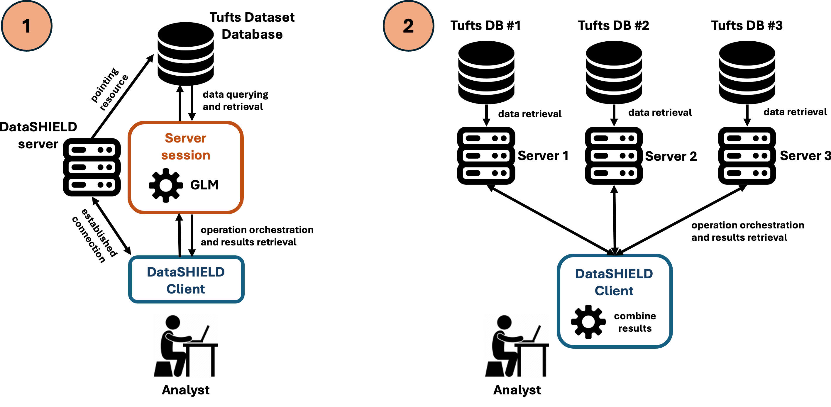
The analysis is conducted using two distinct scenarios to validate the federated approach:
- A centralized analysis using the complete Tufts Synthetic Dataset on a single Opal server.
- A distributed analysis where the dataset is split across three separate Opal servers, each containing a subset of patients, connected through DataSHIELD.
Centralized analysis
Server connection
We start by establishing a connection with ISGlobal’s BRGE development Opal server. This Opal server is configured to allow access to a resource with the full version of the Tufts Synthetic Dataset:
library(DSI)
library(DSOpal)
library(dsBaseClient)
library(dsOMOPClient)
library(dsOMOPHelper)

builder <- newDSLoginBuilder()

builder$append(server="brge",
               url="https://opal.isglobal.org/brge",
               user="dsuser",
               password="P@ssw0rd",
               driver = "OpalDriver")

logindata <- builder$build()
conns <- datashield.login(logins=logindata)
We create an instance of dsOMOPHelper to interact with
the database and build our desired dataset:
o <- ds.omop.helper(
    connections = conns,
    resource = "omop_demo.tufts",
    symbol = "tufts"
)
Dataset construction
Variable definition
We define the variables that will be present in our dataset. These variables include our outcome variable and the predictor variables we will use in our generalized linear model (GLM) for COPD:
Data retrieval
We use dsOMOPHelper’s auto function to
retrieve the defined variables from the tables
condition_occurrence and observation:
Data type conversions
DataSHIELD will not transform an ID to a boolean if it is in a string format, so this process involves two steps:
- Transforming the ID to numeric
- Transforming the numeric ID to boolean
We define a function to perform these steps automatically for every variable:
convert_to_boolean <- function(table, variable_name, id_type, conns) {
  # Construct the full variable name in the format "table$variable_name.id_type"
  full_variable_name <- paste0(table, "$", variable_name, ".", id_type)

  # Create a new variable name for the numeric conversion
  new_numeric_name <- paste0(variable_name, "_numeric")

  # Convert the original variable to numeric
  ds.asNumeric(
    x.name = full_variable_name,
    newobj = new_numeric_name,
    datasources = conns
  )

  # Convert the numeric variable to boolean
  # True (1) if not equal to 0, False (0) otherwise
  # NA values are assigned 0
  ds.Boole(
    V1 = new_numeric_name,
    V2 = 0,
    Boolean.operator = "!=",
    numeric.output = TRUE,
    na.assign = 0,
    newobj = variable_name,
    datasources = conns
  )
}
This allows us to transform the selected variables to boolean format:
# Convert tobacco use observation to boolean
convert_to_boolean("tufts", "tobacco_user",
                   "observation_id", conns)

# Convert condition occurrences to boolean
convert_to_boolean("tufts", "asthma",
                   "condition_occurrence_id", conns)
convert_to_boolean("tufts", "rheumatoid_arthritis",
                   "condition_occurrence_id", conns)
convert_to_boolean("tufts", "vitamin_d_deficiency",
                   "condition_occurrence_id", conns)

# Convert outcome variable (COPD) to boolean
convert_to_boolean("tufts", "chronic_obstructive_pulmonary_disease",
                   "condition_occurrence_id", conns)
## $is.object.created
## [1] "A data object <tobacco_user> has been created in all specified data sources"
##
## $validity.check
## [1] "<tobacco_user> appears valid in all sources"
##
## $is.object.created
## [1] "A data object <asthma> has been created in all specified data sources"
##
## $validity.check
## [1] "<asthma> appears valid in all sources"
##
## $is.object.created
## [1] "A data object <rheumatoid_arthritis> has been created in all specified data sources"
##
## $validity.check
## [1] "<rheumatoid_arthritis> appears valid in all sources"
##
## $is.object.created
## [1] "A data object <vitamin_d_deficiency> has been created in all specified data sources"
##
## $validity.check
## [1] "<vitamin_d_deficiency> appears valid in all sources"
##
## $is.object.created
## [1] "A data object <chronic_obstructive_pulmonary_disease> has been created in all specified data sources"
##
## $validity.check
## [1] "<chronic_obstructive_pulmonary_disease> appears valid in all sources"Create table for the GLM
We create a new table with the prepared outcome and predictors for the GLM:
# We define the name of the variables as they will be in the dataset
variable_names <- c(
  "tobacco_user",
  "asthma",
  "rheumatoid_arthritis",
  "vitamin_d_deficiency",
  "chronic_obstructive_pulmonary_disease"
)

# Create a new table with the prepared outcome and predictors
ds.cbind(
  x = variable_names,
  DataSHIELD.checks = FALSE,
  newobj = "glm_table",
  datasources = conns
)

# Check the structure of the resulting table to ensure it has been created correctly
ds.summary("glm_table")
## $is.object.created
## [1] "A data object <glm_table> has been created in all specified data sources"
##
## $validity.check
## [1] "<glm_table> appears valid in all sources"
##
## $brge
## $brge$class
## [1] "data.frame"
##
## $brge$`number of rows`
## [1] 576750
##
## $brge$`number of columns`
## [1] 5
##
## $brge$`variables held`
## [1] "tobacco_user"
## [2] "asthma"
## [3] "rheumatoid_arthritis"
## [4] "vitamin_d_deficiency"
## [5] "chronic_obstructive_pulmonary_disease"Generalized Linear Model
We can now execute the final step - running the GLM on our prepared dataset:
# Define the formula for the GLM
formula <- paste0(
  "chronic_obstructive_pulmonary_disease ~ ",
  paste(
    c(
      "tobacco_user",
      "asthma",
      "rheumatoid_arthritis",
      "vitamin_d_deficiency"
    ),
    collapse = " + "
  )
)

# Fit the GLM
ds.glm(
  formula = formula,
  data = "glm_table",
  family = "binomial"
)
## $Nvalid
## [1] 576750
##
## $Nmissing
## [1] 0
##
## $Ntotal
## [1] 576750
##
## $disclosure.risk
## RISK OF DISCLOSURE
## brge 0
##
## $errorMessage
## ERROR MESSAGES
## brge "No errors"
##
## $nsubs
## [1] 576750
##
## $iter
## [1] 10
##
## $family
##
## Family: binomial
## Link function: logit
##
##
## $formula
## [1] "chronic_obstructive_pulmonary_disease ~ tobacco_user + asthma + rheumatoid_arthritis + vitamin_d_deficiency"
##
## $coefficients
## Estimate Std. Error z-value p-value
## (Intercept) -6.572083 0.03534378 -185.947355 0.000000e+00
## tobacco_user 1.860760 0.24413811 7.621753 2.502536e-14
## asthma 2.996876 0.11485691 26.092255 4.463685e-150
## rheumatoid_arthritis 2.106862 0.39986610 5.268918 1.372299e-07
## vitamin_d_deficiency 1.814804 0.30800707 5.892084 3.813549e-09
## low0.95CI.LP high0.95CI.LP P_OR
## (Intercept) -6.641355 -6.502810 0.001396927
## tobacco_user 1.382258 2.339262 6.428622994
## asthma 2.771760 3.221991 20.022883190
## rheumatoid_arthritis 1.323139 2.890585 8.222397606
## vitamin_d_deficiency 1.211121 2.418486 6.139869864
## low0.95CI.P_OR high0.95CI.P_OR
## (Intercept) 0.001303556 0.001496976
## tobacco_user 3.983888931 10.373580768
## asthma 15.986751946 25.078005376
## rheumatoid_arthritis 3.755189296 18.003838708
## vitamin_d_deficiency 3.357245312 11.228849381
##
## $dev
## [1] 13173.98
##
## $df
## [1] 576745
##
## $output.information
## [1] "SEE TOP OF OUTPUT FOR INFORMATION ON MISSING DATA AND ERROR MESSAGES"Distributed analysis
Server connection
We start by establishing a connection with the three dedicated Opal servers. Each of these Opal servers contains a resource pointing to a database containing a different subset of the Tufts Synthetic Dataset. In combination, the three Opal servers contain 100% of the original dataset:
builder_dist <- newDSLoginBuilder()

builder_dist$append(server="brge1",
               url="https://opal.isglobal.org/brge1",
               user="dsuser",
               password="P@ssw0rd",
               driver = "OpalDriver")

builder_dist$append(server="brge2",
               url="https://opal.isglobal.org/brge2",
               user="dsuser",
               password="P@ssw0rd",
               driver = "OpalDriver")

builder_dist$append(server="brge3",
               url="https://opal.isglobal.org/brge3",
               user="dsuser",
               password="P@ssw0rd",
               driver = "OpalDriver")

logindata_dist <- builder_dist$build()
conns_dist <- datashield.login(logins=logindata_dist)
We create an instance of dsOMOPHelper to interact with
the three databases. Note that every Opal server will have a different
resource name, so we need to specify the resource for each server:
o <- ds.omop.helper(
    connections = conns_dist,
    resource = list("brge1" = "omop_demo.tufts_dist_1",
                    "brge2" = "omop_demo.tufts_dist_2",
                    "brge3" = "omop_demo.tufts_dist_3"),
    symbol = "tufts_dist"
)
We have specified the symbol tufts_dist for all servers,
so from this point on, we can refer to tufts_dist in each
server and every server will treat it as the same object, despite
containing different parts of the dataset, performing the same
operations on it. Therefore, the analysis will be conducted in the same
way as in the centralized analysis, and DataSHIELD will handle the
distributed nature of the dataset and combine the results.
Dataset construction
Data retrieval
We already had defined the concepts that we want to retrieve under
the outcome_concept_id, condition_list, and
observation_list variables, so we can directly apply the
auto function to the servers. Each server will retrieve the
data for its corresponding part of the dataset:
o$auto(
    table = c("condition_occurrence", "observation"),
    concepts = c(outcome_concept_id, condition_list, observation_list),
    columns = c("condition_occurrence_id", "observation_id")
)
We can observe how the three servers have obtained and stored the
data in their corresponding tufts_dist objects:
ds.summary("tufts_dist", conns_dist)## $brge1
## $brge1$class
## [1] "data.frame"
##
## $brge1$`number of rows`
## [1] 192250
##
## $brge1$`number of columns`
## [1] 16
##
## $brge1$`variables held`
## [1] "person_id"
## [2] "gender_concept_id"
## [3] "year_of_birth"
## [4] "month_of_birth"
## [5] "day_of_birth"
## [6] "birth_datetime"
## [7] "race_concept_id"
## [8] "ethnicity_concept_id"
## [9] "location_id"
## [10] "provider_id"
## [11] "care_site_id"
## [12] "vitamin_d_deficiency.condition_occurrence_id"
## [13] "asthma.condition_occurrence_id"
## [14] "chronic_obstructive_pulmonary_disease.condition_occurrence_id"
## [15] "rheumatoid_arthritis.condition_occurrence_id"
## [16] "tobacco_user.observation_id"
##
##
## $brge2
## $brge2$class
## [1] "data.frame"
##
## $brge2$`number of rows`
## [1] 192250
##
## $brge2$`number of columns`
## [1] 16
##
## $brge2$`variables held`
## [1] "person_id"
## [2] "gender_concept_id"
## [3] "year_of_birth"
## [4] "month_of_birth"
## [5] "day_of_birth"
## [6] "birth_datetime"
## [7] "race_concept_id"
## [8] "ethnicity_concept_id"
## [9] "location_id"
## [10] "provider_id"
## [11] "care_site_id"
## [12] "asthma.condition_occurrence_id"
## [13] "vitamin_d_deficiency.condition_occurrence_id"
## [14] "rheumatoid_arthritis.condition_occurrence_id"
## [15] "chronic_obstructive_pulmonary_disease.condition_occurrence_id"
## [16] "tobacco_user.observation_id"
##
##
## $brge3
## $brge3$class
## [1] "data.frame"
##
## $brge3$`number of rows`
## [1] 192250
##
## $brge3$`number of columns`
## [1] 16
##
## $brge3$`variables held`
## [1] "person_id"
## [2] "gender_concept_id"
## [3] "year_of_birth"
## [4] "month_of_birth"
## [5] "day_of_birth"
## [6] "birth_datetime"
## [7] "race_concept_id"
## [8] "ethnicity_concept_id"
## [9] "location_id"
## [10] "provider_id"
## [11] "care_site_id"
## [12] "asthma.condition_occurrence_id"
## [13] "vitamin_d_deficiency.condition_occurrence_id"
## [14] "chronic_obstructive_pulmonary_disease.condition_occurrence_id"
## [15] "rheumatoid_arthritis.condition_occurrence_id"
## [16] "tobacco_user.observation_id"Data type conversions
The function that we defined previously,
convert_to_boolean, should remain the same. We will apply
it to transform the retrieved data into a boolean format for the
analysis. Each server will apply the function to the data that is stored
in its tufts_dist object:
# Convert tobacco use observation to boolean
convert_to_boolean("tufts_dist", "tobacco_user",
                   "observation_id", conns_dist)

# Convert condition occurrences to boolean
convert_to_boolean("tufts_dist", "asthma",
                   "condition_occurrence_id", conns_dist)
convert_to_boolean("tufts_dist", "rheumatoid_arthritis",
                   "condition_occurrence_id", conns_dist)
convert_to_boolean("tufts_dist", "vitamin_d_deficiency",
                   "condition_occurrence_id", conns_dist)

# Convert outcome variable (COPD) to boolean
convert_to_boolean("tufts_dist", "chronic_obstructive_pulmonary_disease",
                   "condition_occurrence_id", conns_dist)
## $is.object.created
## [1] "A data object <tobacco_user> has been created in all specified data sources"
##
## $validity.check
## [1] "<tobacco_user> appears valid in all sources"
##
## $is.object.created
## [1] "A data object <asthma> has been created in all specified data sources"
##
## $validity.check
## [1] "<asthma> appears valid in all sources"
##
## $is.object.created
## [1] "A data object <rheumatoid_arthritis> has been created in all specified data sources"
##
## $validity.check
## [1] "<rheumatoid_arthritis> appears valid in all sources"
##
## $is.object.created
## [1] "A data object <vitamin_d_deficiency> has been created in all specified data sources"
##
## $validity.check
## [1] "<vitamin_d_deficiency> appears valid in all sources"
##
## $is.object.created
## [1] "A data object <chronic_obstructive_pulmonary_disease> has been created in all specified data sources"
##
## $validity.check
## [1] "<chronic_obstructive_pulmonary_disease> appears valid in all sources"Create table for the GLM
We have successfully prepared the data for the analysis. Now, we can
create a new table with the variables of interest for the GLM. These
variables have already been defined in the variable_names
list previously, so we can directly use it to create the table. This
operation will construct a new table in each server:
# Create new tables with the prepared outcome and predictors
ds.cbind(
  x = variable_names,
  DataSHIELD.checks = FALSE,
  newobj = "glm_table_dist",
  datasources = conns_dist
)

# Check the structure of the resulting tables to ensure they have been created correctly
ds.summary("glm_table_dist", conns_dist)
## $is.object.created
## [1] "A data object <glm_table_dist> has been created in all specified data sources"
##
## $validity.check
## [1] "<glm_table_dist> appears valid in all sources"
##
## $brge1
## $brge1$class
## [1] "data.frame"
##
## $brge1$`number of rows`
## [1] 192250
##
## $brge1$`number of columns`
## [1] 5
##
## $brge1$`variables held`
## [1] "tobacco_user"
## [2] "asthma"
## [3] "rheumatoid_arthritis"
## [4] "vitamin_d_deficiency"
## [5] "chronic_obstructive_pulmonary_disease"
##
##
## $brge2
## $brge2$class
## [1] "data.frame"
##
## $brge2$`number of rows`
## [1] 192250
##
## $brge2$`number of columns`
## [1] 5
##
## $brge2$`variables held`
## [1] "tobacco_user"
## [2] "asthma"
## [3] "rheumatoid_arthritis"
## [4] "vitamin_d_deficiency"
## [5] "chronic_obstructive_pulmonary_disease"
##
##
## $brge3
## $brge3$class
## [1] "data.frame"
##
## $brge3$`number of rows`
## [1] 192250
##
## $brge3$`number of columns`
## [1] 5
##
## $brge3$`variables held`
## [1] "tobacco_user"
## [2] "asthma"
## [3] "rheumatoid_arthritis"
## [4] "vitamin_d_deficiency"
## [5] "chronic_obstructive_pulmonary_disease"Generalized Linear Model
We can now execute the same GLM (with the same formula as in the
centralized analysis, which was defined under the formula
variable previously) on each server:
formula## [1] "chronic_obstructive_pulmonary_disease ~ tobacco_user + asthma + rheumatoid_arthritis + vitamin_d_deficiency"
ds.glm(
  formula = formula,
  data = "glm_table_dist",
  family = "binomial",
  datasources = conns_dist
)
## $Nvalid
## [1] 576750
##
## $Nmissing
## [1] 0
##
## $Ntotal
## [1] 576750
##
## $disclosure.risk
## RISK OF DISCLOSURE
## brge1 0
## brge2 0
## brge3 0
##
## $errorMessage
## ERROR MESSAGES
## brge1 "No errors"
## brge2 "No errors"
## brge3 "No errors"
##
## $nsubs
## [1] 576750
##
## $iter
## [1] 10
##
## $family
##
## Family: binomial
## Link function: logit
##
##
## $formula
## [1] "chronic_obstructive_pulmonary_disease ~ tobacco_user + asthma + rheumatoid_arthritis + vitamin_d_deficiency"
##
## $coefficients
## Estimate Std. Error z-value p-value
## (Intercept) -6.572083 0.03534378 -185.947355 0.000000e+00
## tobacco_user 1.860760 0.24413811 7.621753 2.502536e-14
## asthma 2.996876 0.11485691 26.092255 4.463685e-150
## rheumatoid_arthritis 2.106862 0.39986610 5.268918 1.372299e-07
## vitamin_d_deficiency 1.814804 0.30800707 5.892084 3.813549e-09
## low0.95CI.LP high0.95CI.LP P_OR
## (Intercept) -6.641355 -6.502810 0.001396927
## tobacco_user 1.382258 2.339262 6.428622994
## asthma 2.771760 3.221991 20.022883190
## rheumatoid_arthritis 1.323139 2.890585 8.222397606
## vitamin_d_deficiency 1.211121 2.418486 6.139869864
## low0.95CI.P_OR high0.95CI.P_OR
## (Intercept) 0.001303556 0.001496976
## tobacco_user 3.983888931 10.373580768
## asthma 15.986751946 25.078005376
## rheumatoid_arthritis 3.755189296 18.003838708
## vitamin_d_deficiency 3.357245312 11.228849381
##
## $dev
## [1] 13173.98
##
## $df
## [1] 576745
##
## $output.information
## [1] "SEE TOP OF OUTPUT FOR INFORMATION ON MISSING DATA AND ERROR MESSAGES"As we can observe, the results are the same as in the centralized analysis, but the analysis has been conducted in a distributed manner.
Logout
After finishing the distributed analysis, we close the connections to the servers:
datashield.logout(conns_dist)Conclusion
In this study, we demonstrated the robustness and reliability of
dsOMOP for conducting federated analyses across distributed
datasets. The identical results obtained from both centralized and
distributed approaches validate the effectiveness of our federated
analysis framework. Our findings revealed statistically significant
associations (p < 0.05) between COPD and all examined predictors,
aligning with previously reported relationships in the literature.
These results showcase dsOMOP’s capability to integrate
and analyze distributed medical data while maintaining statistical
integrity. The implementation of this federated approach represents a
significant advancement in distributed clinical data analysis, offering
a solution for large-scale, multi-center studies where data sharing
restrictions may apply.