Part 4: Descriptive analysis
We have already checked that our data is compliant with the codebook. Now we can proceed with our analysis using the selected variables. To begin, we will perform a brief descriptive analysis, calculating some statistics, tables of contingence and doing some graphical visualizations.
Descriptive statistics
There is a collection of DataSHIELD functions to get the descriptive statistics of a variable. Those are the functions ds.var, ds.mean, ds.table among others. However, there is a function from the dsHelper package that automatically performs all the function calls on the background, being a much more user-friendly alternative. The only downside is that it requires the categorical variables to be factors, we can easily create a new factor variable and add it as a new column to our data.
ds.asFactor(input.var.name = "data$CMXHT", newobj.name = "CMXHT_factor")$all.unique.levels
[1] "Yes" "No"
$return.message
[1] "Data object <CMXHT_factor> correctly created in all specified data sources"DSI::datashield.assign.expr(connections, "data", "cbind(data, CMXHT_factor)")
dh.getStats(df = "data", vars = c("DMRAGEYR", "CMXHT_factor"))$categorical
# A tibble: 6 × 10
variable cohort category value cohort_n valid_n missing_n perc_valid
<chr> <chr> <fct> <int> <int> <int> <int> <dbl>
1 CMXHT_factor combined Yes 436 2514 537 1977 81.2
2 CMXHT_factor combined No 101 2514 537 1977 18.8
3 CMXHT_factor sc_verona Yes 285 1515 285 1230 100
4 CMXHT_factor sc_verona No 0 1515 285 1230 0
5 CMXHT_factor umf_cluj Yes 151 999 252 747 59.9
6 CMXHT_factor umf_cluj No 101 999 252 747 40.1
# … with 2 more variables: perc_missing <dbl>, perc_total <dbl>
$continuous
# A tibble: 3 × 15
variable cohort mean std.dev perc_5 perc_10 perc_25 perc_50 perc_75 perc_90
<chr> <chr> <dbl> <dbl> <dbl> <dbl> <dbl> <dbl> <dbl> <dbl>
1 DMRAGEYR sc_vero… 52.1 20.0 16.7 22.4 38 53 68 78
2 DMRAGEYR umf_cluj 63.8 13.0 40.4 46.9 54.2 65 72 80.1
3 DMRAGEYR combined 53.7 19.6 20.1 25.9 40.3 54.7 68.6 78.3
# … with 5 more variables: perc_95 <dbl>, valid_n <dbl>, cohort_n <dbl>,
# missing_n <dbl>, missing_perc <dbl>Graphical visualizations
There is a rich collection of functions to perform graphical visualization of the variables. All the visualizations can be of the pooled data or separated by study.
Boxplot
The boxplot is one of the newest plots available on DataSHIELD. It uses the ggplot2 library, providing lots of customization options.
Combined plot
ds.boxPlot(x = "data", variables = "DMRAGEYR")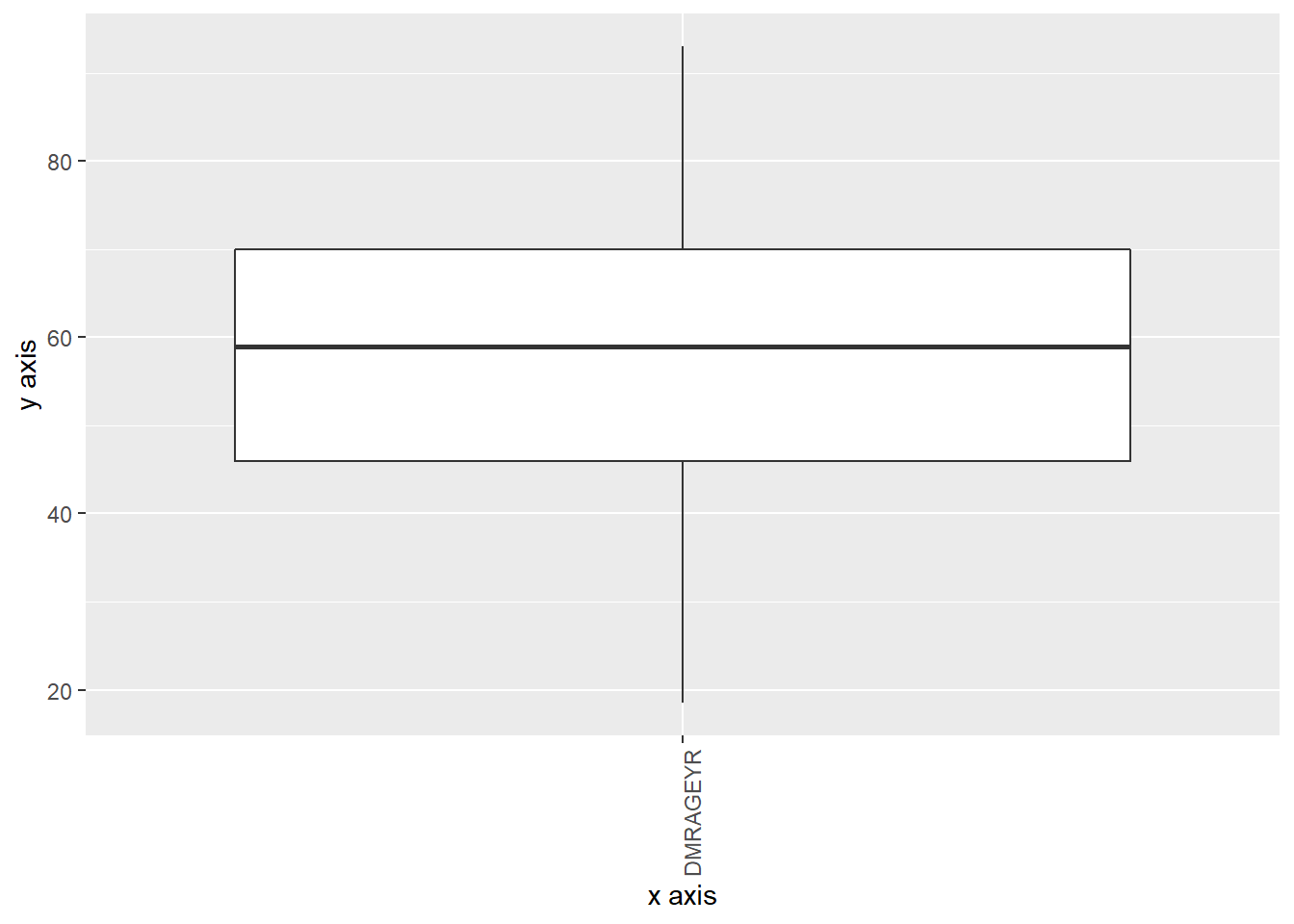
Study separated plot
ds.boxPlot(x = "data", variables = "DMRAGEYR", type = "split")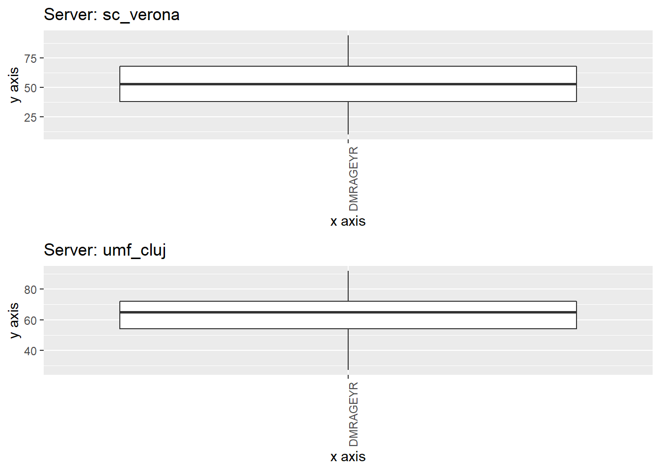
TableGrob (2 x 1) "arrange": 2 grobs
  z     cells    name           grob
1 1 (1-1,1-1) arrange gtable[layout]
2 2 (2-2,1-1) arrange gtable[layout]
Groupings
There are grouping options on the boxplot function which are very useful to have greater insights of the data. We can group using factor variables, so in this example we will use the previously created SMXAPA_factor variable.
ds.boxPlot(x = "data", variables = "DMRAGEYR", group = "CMXHT_factor")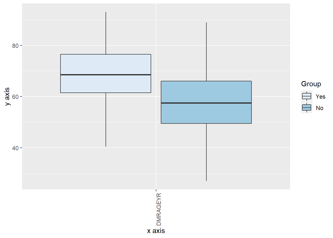
We could even perform a second grouping using the argument group2 and stating another factor variable.
Histogram
To have an idea of the distribution of a variable we can use histograms.
histogram <- ds.histogram("data$DMRAGEYR")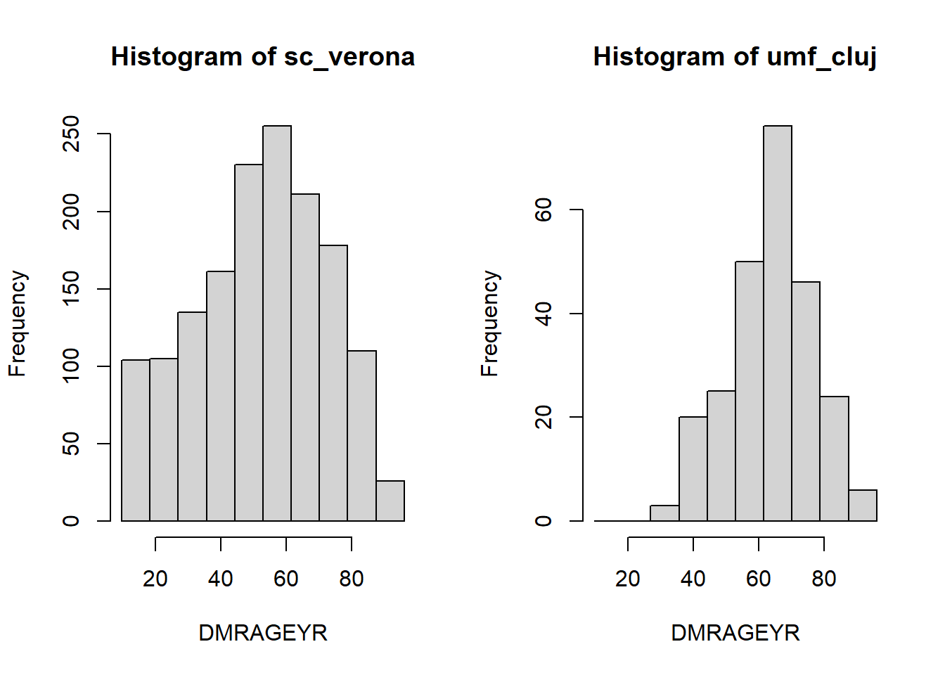
Scatter plot
DataSHIELD has a scatter plot functionality that outputs noise-affected data points, depending on the security configuration of the Opal, the noise levels can make this plot to be hugely distorted.
ds.scatterPlot(x = "data$DMRAGEYR", y = "data$CSXCHRA", datasources = connections)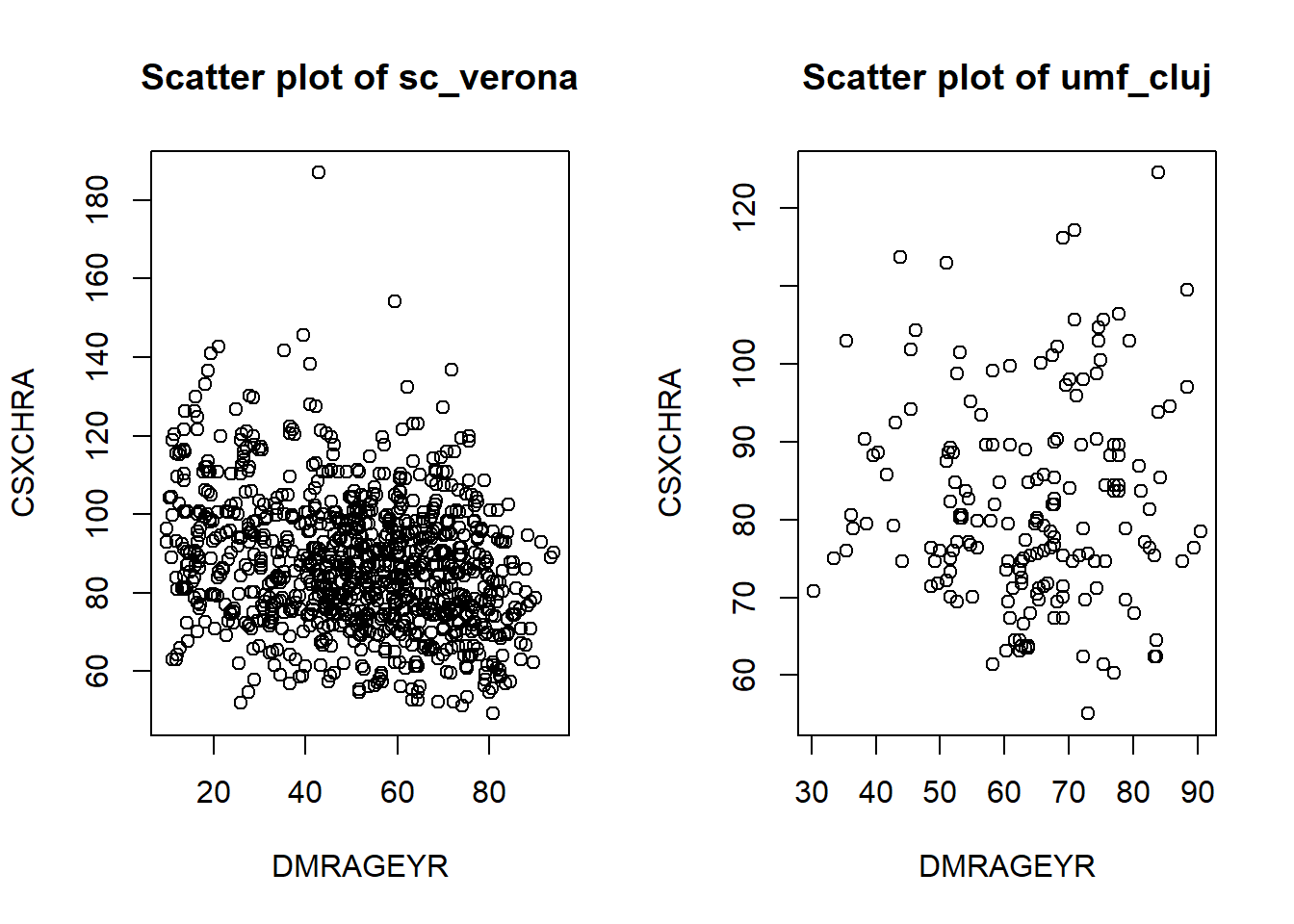
[1] "Split plot created"Heatmap plot
In a similar fashion than the scatter plot, we can visualize a two dimensional distribution of the points but in this case by density.
ds.heatmapPlot(x = "data$DMRAGEYR", y = "data$CSXCHRA")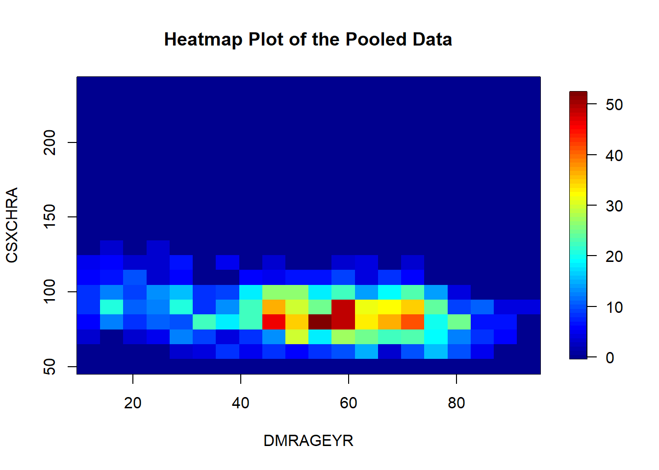
2-Dimensional contingency table
On the previous part, we have already seen that DataSHIELD has a function to calculate uni-dimensional contingency tables. This same function, can also be used for bi-dimensional contingency tables. It is important to note that this function is a little bit tricky sometimes, as it is quite common that the 2D contingency table has disclosive outputs, therefore we just get an error message.
ds.table("data$DMRAGEYR", "data$SMXDIA_numeric")
 All studies failed for reasons identified below


Study 1 :  Failed: at least one cell has a non-zero count less than nfilter.tab i.e. 3

Study 2 :  Failed: at least one cell has a non-zero count less than nfilter.tab i.e. 3
$validity.message
[1] "All studies failed for reasons identified below"
$error.messages
$error.messages$sc_verona
[1] "Failed: at least one cell has a non-zero count less than nfilter.tab i.e. 3"
$error.messages$umf_cluj
[1] "Failed: at least one cell has a non-zero count less than nfilter.tab i.e. 3"There are other variables that do produce valid non-disclosive results.
ctable <- ds.table("data$CMXCVD", "data$CMXCKD")$output.list$TABLES.COMBINED_all.sources_counts
ctable
data$CMXCKD
data$CMXCVD Yes No NA
Yes 20 89 0
No 11 132 0
NA 0 0 747Fisher test
Given the calculated contingency table, we are now in the position to perform a Fisher’s exact test.
stats::fisher.test(ctable)
    Fisher's Exact Test for Count Data

data:  ctable
p-value < 2.2e-16
alternative hypothesis: two.sided
Statistics of a continuous variable grouped by a categorical variable
We may have interest on knowing the value of certain statistics of a variable when grouping with a category. As an example we will calculate the mean of the variable DMRAGEYR (Age) grouped by the variable CMXCOM (Number of comorbidities). Please note this is just an example, those two variables are not expected to be related.
To compute this statistic it is important that we have the categorical variable as a factor, otherwise the grouped statistic calculation will fail. Also, we have to create separate objects for the two variables, we can’t merge them into a data.frame and call them using the typical formulation data.frame$variable, for some reason it fails (to be reported as a bug to the core DataSHIELD team).
ds.assign(toAssign = "data$DMRAGEYR",
            newobj =  "DMRAGEYR")
ds.assign(toAssign = "data$CMXCOM",
            newobj =  "CMXCOM")

ds.tapply(X.name = "DMRAGEYR", INDEX.names = "CMXCOM", FUN.name = "mean")
$sc_verona
$sc_verona$Mean
CMXCOM.0 CMXCOM.1 CMXCOM.2 CMXCOM.3+
46.11960 65.47463 72.60241 78.80000
$sc_verona$N
CMXCOM.0 CMXCOM.1 CMXCOM.2 CMXCOM.3+
1087 335 83 10
$umf_cluj
$umf_cluj$Mean
CMXCOM.0 CMXCOM.1 CMXCOM.2 CMXCOM.3+
53.53125 63.50704 68.98529 70.89362
$umf_cluj$N
CMXCOM.0 CMXCOM.1 CMXCOM.2 CMXCOM.3+
64 71 68 47 This function can take other expressions on the argument FUN.name, more precisely:
"mean""sd""sum""quantile"
Student t-test
We have two options to perform a t-test, and our choice will depend on whether we want to use pooled methods or we want to calculate the t-test on a single study server.
Pooled t-test
To perform a pooled t-test, we will use a collection of DataSHIELD functions to calculate the statistic.
\[t = \frac{\bar{x}_1 - \bar{x}_2}{\sqrt{\frac{s_1^2}{n_1} + \frac{s_2^2}{n_2}}}\]
Where:
- \(\bar{x}\) is the observed mean of the sample.
- \(s\) is the standard devuation of the sample.
- \(n\) is the sample size.
We will use the following code to perform this operations:
mean1 <- ds.mean("data$DMRAGEYR", type = "c")$Global.Mean[1]
mean2 <- ds.mean("data$CSXOSTA", type = "c")$Global.Mean[1]
sd1 <- sqrt(ds.var("data$DMRAGEYR", type = "c")$Global.Variance[1])
sd2 <- sqrt(ds.var("data$CSXOSTA", type = "c")$Global.Variance[1])
n1 <- ds.length("data$DMRAGEYR")[[3]] - sum(unlist(ds.numNA("data$DMRAGEYR")))
n2 <- ds.length("data$CSXOSTA")[[3]] - sum(unlist(ds.numNA("data$CSXOSTA")))

(mean1 - mean2) / sqrt(sd1^2/n1 + sd2^2/n2)
[1] -91.58199You can expect to see a wrapper for this code on a future dsHelper release (dsHelper::dh.ttest('sample1', 'sample2').
Single study t-test
If we are not interested on using pooled functionalities, it is much simpler to perform a t-test.
DSI::datashield.aggregate(connections, "t.test(data$DMRAGEYR, data$CSXOSTA)")$sc_verona
Welch Two Sample t-test
data: data$DMRAGEYR and data$CSXOSTA
t = -88.928, df = 1557.2, p-value < 2.2e-16
alternative hypothesis: true difference in means is not equal to 0
95 percent confidence interval:
-47.07162 -45.03991
sample estimates:
mean of x mean of y
52.06601 98.12177
$umf_cluj
Welch Two Sample t-test
data: data$DMRAGEYR and data$CSXOSTA
t = -31.201, df = 377.97, p-value < 2.2e-16
alternative hypothesis: true difference in means is not equal to 0
95 percent confidence interval:
-30.74986 -27.10393
sample estimates:
mean of x mean of y
63.83200 92.75889 Analysis of variance (ANOVA)
A student is developing a DataSHIELD function to perform ANOVAs. You can expect it to be available in the following months, probably as part of the dsML package.