Heart Failure Mortality Prediction Model Training
End-to-end deep learning workflow for predicting mortality caused by heart failure
Getting Started: Accessing MediNet Hub
What You'll Learn
This use case demonstrates how to train a federated learning model for heart failure mortality prediction using MediNet's platform. You'll learn:
- Complete workflow from dataset selection to model validation
- How to configure and launch federated training
- Understanding training parameters and their impact
- Interpreting performance metrics and optimizing results
Access the Platform
MediNet Hub is accessible through a web interface at:
https://medinet-hub.isglobal.org
(Platform is currently in controlled access for research institutions)
Request credentials:
juanr.gonzalez@isglobal.org
ramon.mateo@isglobal.org
ISGlobal - Barcelona Institute for Global Health
- Your name and institutional affiliation
- Research project description
- Clinical problem you're addressing
- Your role (researcher, clinician, data scientist)
- Username: Your unique researcher identifier
- Password: Secure access credential
- API Key: For programmatic access (if needed)
- Access Permissions: Which datasets you can use
Key Concepts
Before you begin, familiarize yourself with three essential concepts. We'll explain them visually and simply.
What is Federated Learning?
The key principle: Instead of bringing data to the model, we bring the model to the data.
Traditional Centralized Approach
- Hospital A sends patient data → Central Server
- Hospital B sends patient data → Central Server
- Hospital C sends patient data → Central Server
- Server trains model on all centralized data
Privacy violation, slow transfers, expensive storage
Federated Learning Approach
- Hospital A trains the model with its own data
- Hospital B trains the model with its own data
- Hospital C trains the model with its own data
- Only model updates sent back (not data!)
Data stays at source, privacy preserved
Why This Matters
Clinical data is extremely sensitive. Federated learning allows collaboration between hospitals without exchanging actual data, complying with privacy regulations and respecting patient security. This way, you can collaborate with other centers without sharing sensitive information.
What is Differential Privacy?
To further protect privacy, a small level of mathematical "noise" is added to model updates. This works like reinforced anonymization: it's impossible to identify a specific patient even if someone observes the model updates.
The Epsilon (ε) Parameter
The epsilon (ε) parameter controls how much anonymization is added to protect patient privacy.
Example: Understanding Differential Privacy with Salaries
Scenario: A hospital wants to publish average doctor salaries without revealing individual salaries.
Without Differential Privacy: If you know all salaries except one, you can calculate the missing one exactly.
With Differential Privacy: Add random noise to the average (e.g., ±$2,000). Now even if you know all other salaries, you cannot determine the exact missing salary—only approximate it within a range.
In federated learning: The same principle applies to model weights. Noise is added so that individual patient contributions cannot be extracted from the trained model.
What are Neural Networks?
A neural network works like a set of layers that process information step by step:
- They receive patient data
- They learn patterns internally
- They produce a final prediction
They're well-suited for clinical problems because they can learn complex relationships between variables.
What is a neuron? A neuron is the basic processing unit in a neural network. Similar to neurons in the brain, artificial neurons receive inputs (like patient data), process them using mathematical operations, and produce an output. Multiple neurons work together in layers to detect increasingly complex patterns in the data.
Neural Network Architecture Basics
Input Layer
Patient features
Hidden Layer 1
64 neurons (ReLU)
Hidden Layer 2
32 neurons (ReLU)
Output Layer
1 neuron (Sigmoid)
- Input Layer: Receives patient data (age, lab results, etc.)
- Hidden Layers: Extract progressively complex patterns (64 neurons → 32 neurons)
- Activation Functions (ReLU): Allow network to learn non-linear relationships
- Output Layer: Produces final prediction (mortality risk: 0 to 1)
How Neural Networks Learn
Neural networks learn by adjusting connection weights between neurons. During training, the network makes predictions, calculates how wrong they are (loss), and updates weights to improve. This process repeats thousands of times (epochs) until the network learns accurate patterns in the data.
Process Flow
The training process follows a structured workflow from authentication to final model validation:
How to Access MediNet
Let's begin our journey with MediNet. We'll start by accessing the platform and authenticating.
- We open our browser and navigate to the MediNet platform using the provided link.
- Next, we enter our credentials (username, password) in the login form.
- We click Login and wait for authentication.
- Once logged in, we're greeted by the main dashboard—our control center for managing datasets, connections, and training projects.
Don't have credentials yet? See how to request access at the beginning of this guide.
This is our essential first step before continuing with the federated learning workflow.
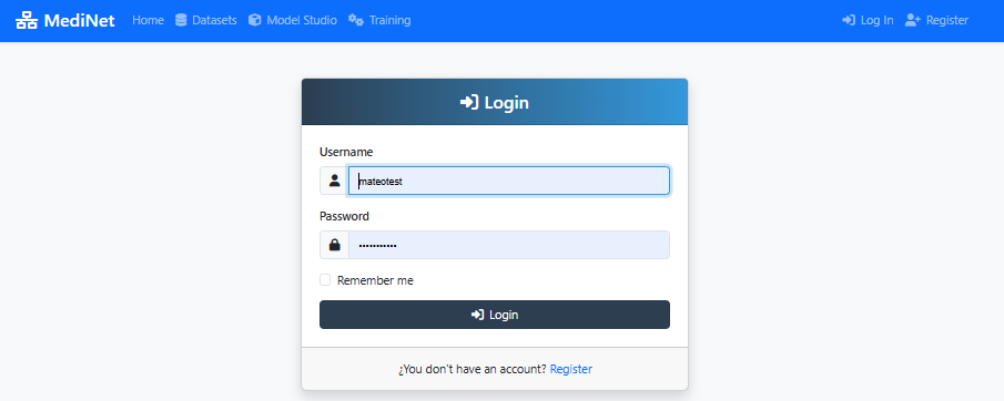
Figure 1: MediNet login screen - enter your credentials to access the platform
What You Should See
In the screenshot above (Figure 1), observe:
- Two input fields: Username, Password
- Login button: Prominently displayed at the bottom
- MediNet branding: Logo and welcome message at the top
✅ After successful login: You'll be redirected to the main dashboard showing "Welcome, [your name]" and navigation menu on the left.
Connect to MediNet Nodes and Select Datasets
Now that we've successfully logged in and accessed the main dashboard, our next step is to connect to the data node where the clinical records are stored. Remember: in federated learning, the data never leaves its original location.
Adding a Node Connection
- From the Right side menu, we click on Datasets.
- We select Add Connections from the dropdown.
- We click the Add New Connection button.
- We enter the connection details provided by the data administrator:
- Connection name
- IP address
- Port
- Username
- Password
- API Key
- We click Test Connection to verify connectivity with the node.
- Once the test succeeds (showing a green checkmark ✅), we click Sincronize icon to get the datasets available in MediNet Node that we added.
Selecting the Dataset
- With our node connection established, we navigate to the Datasets section.
- We locate the heart_failure_clinical_records dataset in the list.
- We click on it to open the dataset details panel.
- We carefully review the available information: variables, data types, number of samples, and target feature.
Understanding the Power of Federated Learning: In a real federated deployment, this type of clinical data exists at multiple hospitals. Instead of centralizing data (privacy violation), MediNet enables collaborative training where the model travels to the data.
Federated Learning Scenario
Imagine three hospitals collaborating:
- Hospital A: 500 heart failure patients (urban, younger population)
- Hospital B: 800 heart failure patients (rural, older population)
- Hospital C: 600 heart failure patients (diverse demographics)
Model learns from all 1,900 patients while data never leaves each hospital
Dataset Characteristics
Why This Dataset?
This dataset demonstrates a typical healthcare prediction task: binary classification with mixed features. The workflow you'll learn applies to any medical prediction problem: disease diagnosis, treatment response, patient risk stratification, readmission prediction, etc.
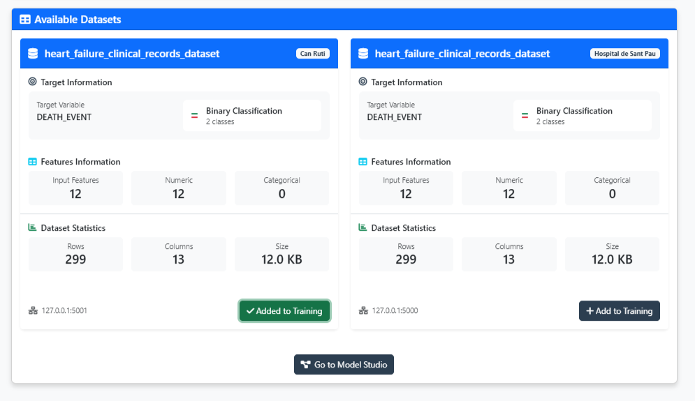
Figure 2: Dataset explorer - validate your data is ready for training
What You Should See
In the dataset explorer (Figure 2), you should observe:
- Dataset name: "heart_failure_clinical_records"
- Number of samples: 8762 patients
- Number of Rows: 12 clinical variables
- Target variable: Heart Attack Risk (binary: 0=No risk, 1=Risk)
- Feature types: Mix of continuous (age, Cholesterol, Heart Rate) and binary(Hemisphere_Northern, Previous Heart Problems)
✅ Validation check: If you see "Added to training" with a green indicator, the dataset has been properly added on the configuration and you can proceed to model design.
Navigate to Model Studio
Now that we've selected our dataset, it's time to create the neural network architecture. But first, we need to navigate to Model Studio—MediNet's workspace for managing and designing AI models.
Accessing Model Studio
- After validating the dataset, we click the "Go to Model Studio" button located at the bottom of the dataset explorer.
- This takes us to the Model Studio interface—our central hub for all model-related activities.
What is Model Studio? This workspace lets you browse existing models, create new architectures, compare model performance, and import pre-trained models. Think of it as your model library and design center.
Creating a New Model
Once in Model Studio, we'll see the model management interface. Since this is our first model, the workspace will be empty with a message: "No models found - Create your first model to get started."
- We click either the "Create Model" button in the center or the "+ New Model" button in the top-right corner.
- A dialog appears asking: "What kind of model would you like to create?"
- We see three options:
- Sequential Model: Build linear sequential neural networks (perfect for our use case)
- Advanced Model (Residual Connections): Build complex architectures with skip connections (ResNet, U-Net, etc.)
- Machine Learning Model: Configure classic algorithms like SVM, Random Forest, etc.
- For our heart failure mortality prediction, we select "Sequential Model"—the most straightforward approach for tabular clinical data.
Ready to design! Clicking "Sequential Model" opens the visual Model Designer where we'll build our architecture layer by layer.
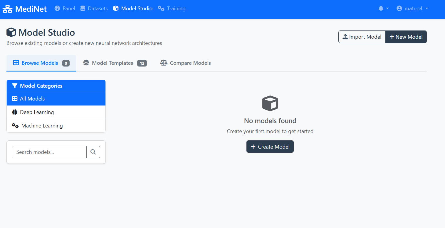
Figure 3a: Model Studio - your workspace for managing AI models
What You Should See
In the Model Studio interface (Figure 3a), observe:
- Navigation tabs: "Browse Models" (0), "Model Templates" (12), "Compare Models"
- Left sidebar: Model Categories (All Models, Deep Learning, Machine Learning)
- Empty workspace message: "No models found" with a cube icon
- Action buttons: "Import Model" and "+ New Model" in the top-right
- Create Model button: Centrally placed for easy access
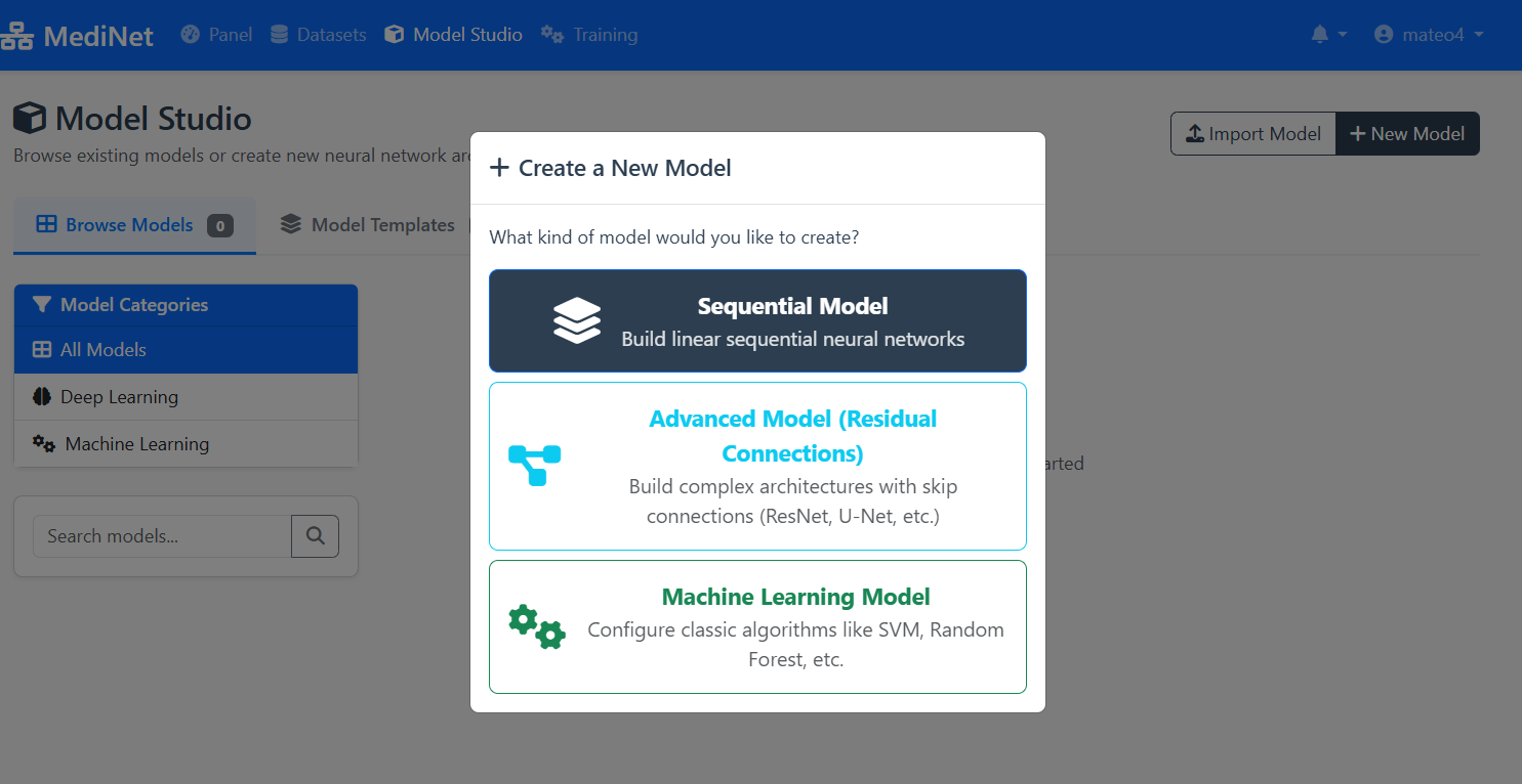
Figure 3b: Model type selection - choosing Sequential Model for our use case
What You Should See
In the model creation dialog (Figure 3b), observe:
- Dialog title: "+ Create a New Model"
- Sequential Model (top, selected): Dark background with layers icon - "Build linear sequential neural networks"
- Advanced Model (middle): Cyan text with connection icon - For ResNet, U-Net architectures
- Machine Learning Model (bottom): Green text with gears icon - For SVM, Random Forest, etc.
✅ Selection confirmed: Click "Sequential Model" to proceed to the visual Model Designer interface.
Create the Model in Model Designer
Now that we've selected and explored our dataset, let's move to the exciting part: designing the neural network architecture. With MediNet's visual Model Designer, we can build sequential models without writing a single line of code.
Opening the Designer
- From the left navigation menu, we click on Model Studio.
- We select Model Designer from the submenu.
Building the Architecture
- We click the Add Layer button in the designer canvas.
- We add an input layer (this auto-configures based on our selected dataset—52 features in this case).
- Next, we add a hidden layer with 12 input neurons and 64 output neurons and added a after a ReLU activation layer.
- We add another hidden layer with 64 input neuronas and 32 output neurons, again adding a ReLU activation layer.
- Finally, we added an last hidden layer with 32 input neurons and 1 output neuron (Activation layer on th
Configuring Optimizer and Loss Function
After building the architecture, we need to configure how the model will learn. In the Model Configuration panel, we set:
- We select Adam as the optimizer (handles learning rate adaptation automatically)
- We set the Learning Rate to 0.001 (standard starting point for Adam)
- We choose Binary Cross Entropy with Logits as the loss function (appropriate for binary classification)
- We click Save to store our complete model configuration.
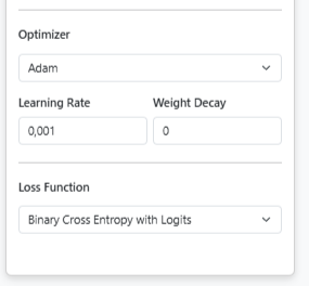
Model Configuration Panel: Setting optimizer and loss function
Want to learn more? For detailed explanations about optimizers, loss functions, and other training parameters, see Step 5: Training Parameters Explained. You can also explore other optimizer options in the PyTorch documentation.
The model is now ready to be trained.
Model Configuration Used in This Use Case
Architecture:
Input Layer: Matches dataset features (automatically configured)
Hidden Layer 1: 64 neurons with ReLU activation
Hidden Layer 2: 32 neurons with ReLU activation
Output Layer: 1 neuron with Sigmoid activation (binary classification)
Training Configuration:
Optimizer: Adam (adaptive learning with momentum)
Learning Rate: 0.001
Loss Function: Binary Cross-Entropy with Logits
Visual Designer
Click "Add Layers" button to build neural network architecture without coding
Layer Configuration
Define activation functions, neuron counts, and connections between layers
Save Configuration
Click "Save" to store your model - you can modify it later
Pedagogical Focus
This architecture demonstrates MediNet's capabilities, not clinical optimization. The simple 64→32 structure is intentionally chosen to show how easy it is to design neural networks visually.
In real research: You would iterate on architecture, try different sizes, add regularization (dropout), experiment with depths—all visually through MediNet's interface without coding.
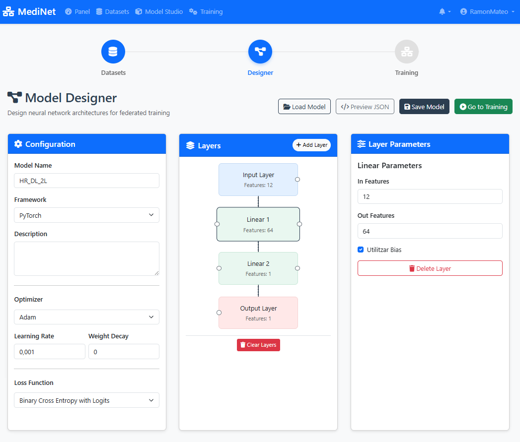
Figure 4: Visual Model Designer - build your AI architecture with drag-and-drop
What You Should See
In the Model Designer interface (Figure 4), you should observe:
- Visual canvas: A drag-and-drop workspace showing layer blocks connected vertically
- Layer stack: Input(12) → Dense(64, ReLU) → Dense(32, ReLU) → Output(1, Sigmoid)
- Add Layer button: Located at the top or side of the canvas
- Layer properties panel: Displays neuron count and activation function for each selected layer
- Save button: Prominently displayed (typically top-right corner)
✅ Architecture confirmation: When saved successfully, you'll see "Model architecture saved" with a green checkmark and the model name will appear in your Models list.
Configure Training
With our model architecture defined, we now need to configure how it will learn. This is where we set the training hyperparameters that control the learning process. MediNet provides explanatory tooltips for each parameter as we configure them.
- From the left menu, we navigate to Training.
- We select the model we just created from the dropdown list.
- We configure the training parameters:
- Learning Rate: 0.001
- Local Epochs: 20
- Federation Rounds: 10
- Loss Function: Binary Cross-Entropy
- Batch Size: 32
As you configure each parameter, you'll see an explanatory panel that helps you understand its effect.
Training Parameters Explained
What it controls: The magnitude of weight updates during training. It determines how aggressively the model adjusts its parameters after seeing each batch of data.
Why Learning Rate Matters - Click to Expand
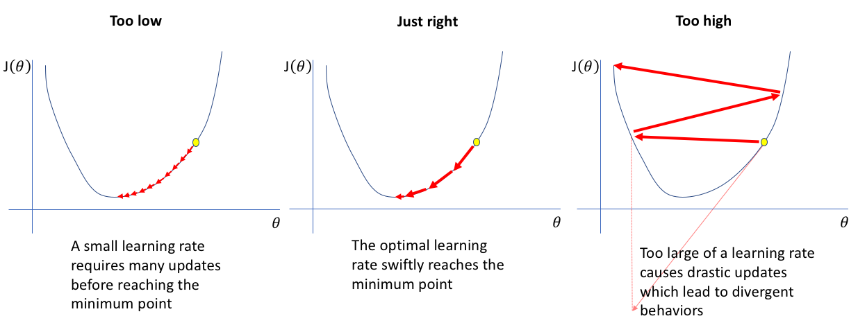
Too Low: The model takes tiny steps towards the optimal solution. Training is very slow, requiring many iterations to converge. May get stuck in local minima.
Just Right: The model efficiently navigates toward the optimal solution with appropriate step sizes. Balances speed and stability.
Too High: The model takes overly large steps, overshooting the optimal solution and bouncing around. Training becomes unstable and may diverge entirely.
Common starting points: Standard learning rates like 0.01 or 0.001 are typically good starting values. These provide a balance between convergence speed and stability for most problems. In practice, you monitor training curves and adjust if the loss oscillates (too high) or converges too slowly (too low).
What it controls: How many complete passes the model makes through the local dataset at each participating hospital in federated learning.
In this use case: We'll use 20 local epochs per federation round.
Understanding Local Epochs - Click to Expand
Trade-off: More epochs allow better local learning, but excessive epochs risk overfitting to local data before global aggregation.
In federated learning: We typically use fewer local epochs (10-20) than centralized training because the model gets updated multiple times through federation rounds.
Recommended range: 10-20 epochs per round for most federated learning tasks
What it controls: The number of times the global model is distributed to participating sites, trained locally, and aggregated back. This is the key parameter that distinguishes federated learning from centralized training.
Understanding Epochs vs Rounds - Click to Expand
Round 1:
- Coordinator sends initial model to all hospitals
- Hospital A trains for 20 epochs on local data → sends updates
- Hospital B trains for 20 epochs on local data → sends updates
- Hospital C trains for 20 epochs on local data → sends updates
- Coordinator aggregates updates → Global Model v1
Round 2:
- Coordinator sends Global Model v1 to all hospitals
- Each hospital trains for 20 more epochs → sends updates
- Coordinator aggregates → Global Model v2
... continues for N rounds
Total training: 10 rounds × 20 local epochs = 200 total epochs of learning at each site, but with cross-hospital knowledge sharing after every 20 epochs
Trade-offs:
- Many rounds, few local epochs: Frequent aggregation, faster global convergence, more communication
- Few rounds, many local epochs: Less communication, but risk of local overfitting
- Balanced (10 rounds × 20 epochs): Standard starting point
In this use case: We'll configure 10 federation rounds.
What it controls: The mathematical function used to quantify how far the model's predictions are from the true values. The training process minimizes this loss.
In this use case: Binary Cross-Entropy is used because we're predicting a binary outcome (death event: yes/no).
Common Loss Functions - Click to Expand
Binary Cross-Entropy: For binary classification (death/survival). Measures the difference between predicted probabilities and actual binary outcomes.
Categorical Cross-Entropy: For multi-class classification (3+ categories). Generalizes binary cross-entropy to multiple classes.
Mean Squared Error (MSE): For regression tasks (predicting continuous values). Penalizes larger errors more heavily than smaller ones.
What it controls: How many samples the model processes before updating its weights. The dataset is divided into batches, and weights are updated after each batch.
Understanding Batch Size Impact - Click to Expand
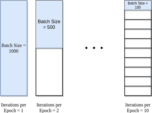
Understanding the visualization: The diagram above shows a dataset with 1000 total samples (e.g., 1000 patient records). The batch size determines how these samples are divided for processing.
Batch Size = 1000 (entire dataset): All 1000 samples processed together = 1 iteration per epoch. This is like setting batch size equal to your entire dataset size. Fast computation but only one weight update per epoch, which means very slow learning.
Batch Size = 500 (half dataset): 1000 samples ÷ 500 batch size = 2 iterations per epoch. Two weight updates per epoch provides more learning opportunities while maintaining computational efficiency.
Batch Size = 100 (1/10th dataset): 1000 samples ÷ 100 batch size = 10 iterations per epoch. Many weight updates provide frequent learning opportunities but with noisier gradients. Often leads to better generalization.
Memory Consideration: Larger batches require more GPU/CPU memory. If you encounter out-of-memory errors, reduce the batch size.
Practical tip: Common batch sizes are 16, 32, 64, 128, or 256. The choice depends on your dataset size and available memory. For our heart failure dataset, the batch size was selected to balance training speed, memory constraints, and gradient quality.
What it controls: The optimization algorithm that adjusts the model's weights based on the computed loss. The optimizer determines how the model learns from its mistakes.
In this use case: We use Adam (Adaptive Moment Estimation) because it adapts the learning rate for each parameter automatically and works well across a wide range of problems without extensive tuning.
Why Adam for This Use Case - Click to Expand
Adam advantages:
- Adaptive learning rates: Automatically adjusts step sizes for different parameters
- Momentum: Uses past gradients to smooth out updates and accelerate convergence
- Robust: Works well with sparse gradients and noisy data (common in clinical datasets)
- Minimal tuning: Default hyperparameters (β₁=0.9, β₂=0.999) work well for most cases
Other available optimizers:
- SGD (Stochastic Gradient Descent): Simple and stable, but may require more careful learning rate tuning. Good when you need more control.
- RMSprop: Good for recurrent neural networks and non-stationary problems. Adapts learning rates based on recent gradients.
Learn more: For detailed information about these optimizers and their parameters, see the PyTorch documentation:
Adam optimizer
SGD optimizer
RMSprop optimizer
Configuration Used in This Use Case
The researcher configured the following parameters for federated training:
- Optimizer: Adam (adaptive learning with momentum)
- Learning Rate: 0.001 (standard starting point for Adam optimizer)
- Local Epochs: 20 (passes through local data per round)
- Federation Rounds: 10 (global aggregation cycles)
- Loss Function: Binary Cross-Entropy (binary classification)
- Batch Size: 32 (balances training stability and generalization)
Total training computation: 10 rounds × 20 epochs = 200 total local epochs per participating hospital
Note: These parameters may require adjustment based on your specific dataset, computational resources, and model architecture.
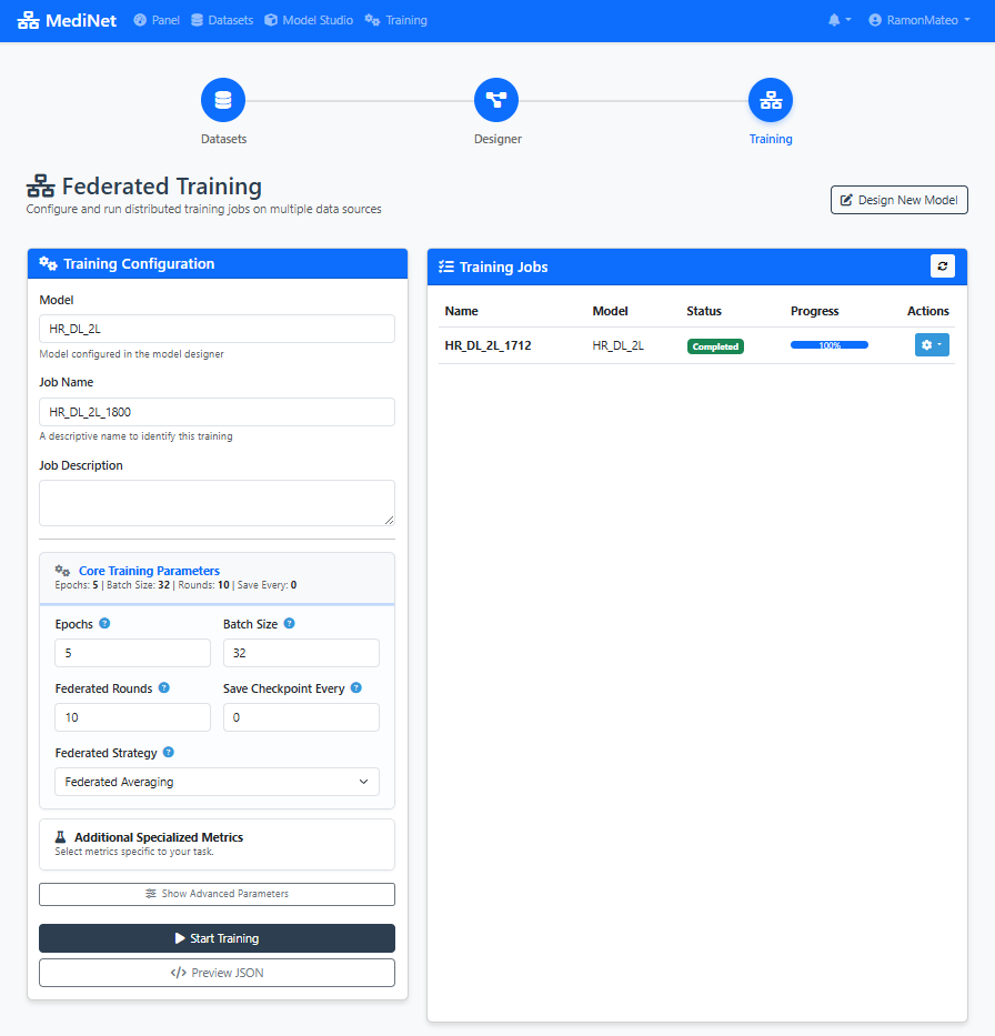
Figure 5: Training configuration panel - set your learning parameters with recommended values
What You Should See
In the Training Configuration panel (Figure 5), you should observe:
- Model selection dropdown: Shows your saved model (e.g., "heart_failure_predictor")
- Hyperparameter input fields: Learning Rate (0.001), Local Epochs (20), Federation Rounds (10), Batch Size (32)
- Loss function selector: "Binary Cross-Entropy" selected for binary classification
- Info icons (ⓘ): Next to each parameter providing explanatory tooltips
- Start Training button: Disabled until all required fields are filled
✅ Configuration ready: When all parameters are set, the "Start Training" button turns green, indicating we can proceed to training execution.
Execute Training
Now comes the moment we've been building toward: launching the federated training process. With our configuration set, we're ready to start training across multiple hospital nodes simultaneously. This is where we witness federated learning in action.
- We click the Start Training button to initiate the federated learning process.
- The interface automatically switches to the Results / Analysis tab, where we can monitor progress in real-time.
- During training, we observe several key metrics updating dynamically:
- Loss curves: Both training and validation loss plotted over rounds
- Accuracy metrics: Training and validation accuracy percentages
- Round progression: Current round number and completion status
- Time metrics: Time per epoch and estimated completion time
Interpreting the metrics:
- If the loss oscillates too much, the learning rate may be too high.
- If validation diverges, there may be overfitting.
Performance Metrics
Loss
Training and validation loss curves
Accuracy
Model prediction accuracy over epochs
Error Metrics
Additional performance measurements
Model Performance Comparison
Comparison of model accuracy across different batch sizes:
| Configuration | Batch Size | Accuracy | Status |
|---|---|---|---|
| Initial Model | 16 | 53.64% | 📊 Baseline |
| Optimized Model | 32 | 54.30% | ✅ Improved |
⚠️ If your values diverge significantly:
• Loss oscillating wildly? Learning rate may be too high (reduce to 0.0005)
• Validation loss increasing? Possible overfitting (reduce local epochs or add regularization)
• Accuracy stuck below 70%? Model may need more complexity or different architecture
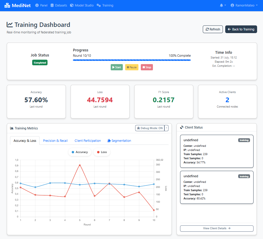
Figure 6: Real-time monitoring dashboard with loss, accuracy, and performance metrics
What You Should See
In the real-time training dashboard (Figure 6), you should observe:
- Round progress indicator: "Round 1/10 completed" at the top
- Loss graph (left panel): Two curves showing training loss (red/orange) and validation loss (blue) decreasing over rounds
- Accuracy panel (right): Training and validation accuracy percentages increasing over rounds
- Status messages: "Training in progress..." or "Round X completed successfully"
- Time estimates: "Estimated time remaining: X minutes"
✅ Training complete: When all 10 rounds finish, you'll see "Training completed successfully" with a green checkmark. The final model is automatically saved and ready for evaluation or deployment.
Optimize Performance
With our first training complete and metrics in hand, we now enter the iterative optimization phase. This is where we refine our model by analyzing results and making informed adjustments to improve performance.
Observe the Metrics
- We carefully review the displayed metrics from our initial training run.
- If we detect possible improvements (e.g., high loss oscillation, slow convergence), we navigate back to the Training configuration panel.
- We adjust only one parameter at a time (for example, batch size) to isolate its effect.
- We launch a second training iteration with the modified parameter.
- We compare the results between the first and second runs side by side.
This fine-tuning process is key to improving model quality.
Interpreting Training Metrics
Loss Curve Analysis: If loss decreases steadily and plateaus, training is progressing well. If it oscillates wildly, learning rate may be too high.
Training vs Validation Gap: Large gap indicates overfitting - model memorizes training data but doesn't generalize. Consider reducing epochs or model complexity.
Training Speed: If each epoch takes too long, consider increasing batch size (if memory allows) or simplifying the architecture.
In this example: The researcher analyzes the metrics from initial training and decides to adjust the batch size to optimize convergence behavior.
Hyperparameter Optimization
Why Adjust Parameters? Based on the analysis, the researcher identifies that modifying the batch size could improve training behavior - either speeding up convergence or improving generalization.
Rationale: Adjust the trade-off between training speed and gradient noise. The new value was selected to optimize convergence behavior for this specific dataset size.
Next Step: Launch a new training cycle with the adjusted hyperparameters and compare the resulting metrics against the previous run.
Iterative Optimization Best Practices
- Change ONE parameter at a time to isolate the effect of each adjustment
- Document each configuration and its results for comparison
- Use validation metrics (not training metrics) to guide decisions
- Be patient - small improvements compound over iterations
- Stop iterating when validation performance plateaus or begins to degrade
Second Training Cycle
The model is retrained with batch size set to 32. MediNet monitors the training process and generates updated performance metrics.
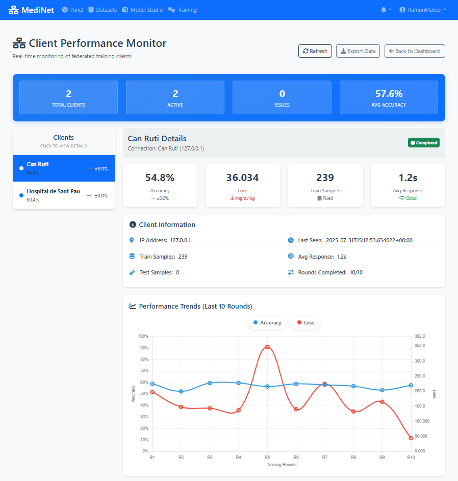
Figure 7: Performance comparison: initial training vs. optimized training with batch size 32
Final Model Validation
When we're satisfied with the performance after our optimization iterations, we perform final validation checks:
- We check that the loss has stabilized and is no longer decreasing significantly.
- We verify that accuracy metrics are consistent across training and validation sets.
- We ensure there's no overfitting (validation loss not diverging from training loss).
- Finally, we mark the model as Valid within the platform, making it ready for deployment or clinical validation.
The model is ready for clinical use or additional validation.
Quick Validation Reference
Final Artifact
Validated Deep Learning Model for cardiac risk prediction, ready for deployment or further clinical validation.
Exportable Configuration (JSON)
Throughout this tutorial, MediNet has been generating a JSON configuration file in the background. This file captures your entire workflow—model architecture, training parameters, dataset references—and can be exported for reproducibility or sharing with colleagues.
{
    "metadata": {
        "version": "1.0",
        "created_at": "2025-11-20T11:50:16.211Z",
        "model_type": "dl_linear",
        "framework": "pytorch"
        },
    "basic_info": {
        "name": "Model1",
        "description": ""
    },
    "architecture": {
        "layers": [
            {
                "name": "Input Layer",
                "type": "input",
                "params": {
                    "features": 52
                },
                "readonly": true
            },
            {
                "name": "Linear",
                "type": "Linear",
                "params": {
                    "in_features": 52,
                    "out_features": 64,
                    "bias": true,
                    "features": 64
                }
            },
            {
                "name": "ReLU",
                "type": "ReLU",
                "params": {
                    "features": 64
                }
            },
            {
                "name": "Linear",
                "type": "Linear",
                "params": {
                    "in_features": 64,
                    "out_features": 1,
                    "bias": true,
                    "features": 1
                }
            },
        {
            "name": "Output Layer",
            "type": "output",
            "params": {
                "features": 1
            },
            "readonly": true
        }
        ]
    },
    "training": {
        "optimizer": {
            "type": "adam",
            "learning_rate": 0.001,
            "weight_decay": 0,
            "differential_privacy": {
                "noise_multiplier": 1,
                "max_grad_norm": 1,
                "random_seed": 42
            }
        },
        "loss_function": "bce_with_logits",
        "metrics": [],
        "epochs": 5,
        "batch_size": 32,
        "rounds": 10,
        "flower_version": "1.6"
    },
    "dataset": {
        "selected_datasets": [
            {
                "dataset_id": "2",
                "dataset_name": "Hearth Atack Risk ",
                "features_info": {
                "input_features": 52,
                "feature_types": {
                    "numeric": 23,
                    "categorical": 30
                }
            },
            "target_info": {
                "name": "Heart Attack Risk",
                "type": "classification",
                "task_subtype": "binary_classification",
                "data_type": "numeric",
                "num_classes": 2,
                "classes": [
                0,
                1
                ],
                "output_neurons": 1,
                "recommended_activation": "sigmoid",
                "recommended_loss": "BCEWithLogitsLoss"
            },
                "num_columns": 53,
                "num_rows": 8762,
                "size": 2526628,
                "connection": {
                    "name": "can ruti",
                    "ip": "127.0.0.1",
                    "port": "5001"
                }
            }
        ]
    },
    "federated": {
        "name": "FedAvg",
        "parameters": {
            "fraction_fit": 1,
            "fraction_eval": 0.3,
            "min_fit_clients": 1,
            "min_eval_clients": 1,
            "min_available_clients": 1
        }
    },
    "job_config": {
        "job_name": "Model1_1246",
        "job_description": "",
        "save_frequency": 0
    }
}
How to Export:
- Navigate to Training → Results
- Click the Export Configuration button (top-right corner)
- The JSON file downloads automatically as
heart_failure_predictor_config.json
Future capability: In upcoming MediNet versions, you'll be able to directly import and edit JSON configuration files to quickly recreate or modify training experiments.
Platform Features & Benefits
Complete workflow from dataset to validated model
Dataset Management
Secure access to pre-processed medical datasets with metadata validation and exploration capabilities.
Visual Model Designer
Intuitive drag-and-drop interface for designing deep learning architectures without coding.
Hyperparameter Configuration
Comprehensive control over training parameters including learning rate, epochs, loss functions, and batch size.
Training Execution
Automated training workflow with real-time monitoring and performance tracking.
Performance Analysis
Detailed metrics visualization including loss curves, accuracy charts, and error measurements.
Iterative Optimization
Support for multiple training cycles with hyperparameter tuning and performance comparison.
Data Privacy
Medical data remains at Hospital X while enabling model training through federated learning architecture.
No Coding Required
Researchers can design and train complex deep learning models using visual interfaces without programming knowledge.
Fast Experimentation
Quick iteration cycles enable researchers to optimize models efficiently through hyperparameter tuning.
Clinical Validation
Structured workflow from training to validation ensures models meet clinical requirements before deployment.
Ensuring transparent, verifiable, and replicable research
Platform Version
MediNet v0.1.x
Released: November 2025
Dataset Version
heart_attack_prediction_dataset
Preprocessed & validated
Download Datasets
Raw: 8764 samples | Preprocessed: one-hot encoded
Complete Configuration Package
The exported JSON configuration (shown in Step 6) contains all parameters needed to reproduce this experiment. Combined with the platform and dataset versions listed above, any researcher can replicate these results exactly.
For complete installation instructions and environment setup, refer to our comprehensive guide:
MediNet Installation Guide