Validation Study: Centralized vs. Federated Vertical Analysis

David Sarrat González

Introduction

This vignette presents a comparative validation of the dsVert federated vertical analysis pipeline against centralized R computations. We exercise the full protocol stack — ECDH-PSI record alignment, MHE-CKKS correlation, spectral PCA, and encrypted-label GLMs — on real data vertically partitioned across three DataSHIELD servers.

The study is organized in three parts:

1. Federated vertical analysis — PSI alignment followed by correlation, PCA, and GLMs computed via dsVert, where each server holds a different subset of variables and no raw data leaves any server.
2. Centralized analysis — ground truth computed with standard R functions on the matched cohort.
3. Comparative assessment — side-by-side numerical comparison with error analysis.

Dataset

We use a modified version of the Pima Indian women diabetes training set (Pima.tr, $n = 200$) from the MASS R package (Venables & Ripley, 2002). It contains clinical measurements for 200 women of Pima heritage aged $\geq 21$ years, collected by the US National Institute of Diabetes and Digestive and Kidney Diseases near Phoenix, Arizona (Smith et al., 1988). Seven numeric variables are available: npreg (number of pregnancies), glu (plasma glucose), bp (diastolic blood pressure), skin (triceps skin fold thickness), bmi (body mass index), ped (diabetes pedigree function), and age (years).

Data preparation and vertical partitioning

We load the dataset from MASS::Pima.tr, assign patient identifiers, and partition it into three vertical fragments with deliberately non-identical patient populations. This simulates a realistic scenario where institutions have data on overlapping but non-identical patient cohorts.

library(MASS)
data("Pima.tr", package = "MASS")
df <- as.data.frame(Pima.tr)
df$patient_id <- sprintf("P%03d", seq_len(nrow(df)))
df$diabetes   <- ifelse(df$type == "Yes", 1L, 0L)

set.seed(123)

# 150 patients are shared across all 3 servers (the "common core")
core_ids <- sample(df$patient_id, 150)
remaining <- setdiff(df$patient_id, core_ids)

# Each server gets the core + a different subset of extras
ids1 <- sample(c(core_ids, sample(remaining, 30)))  # 180 patients
ids2 <- sample(c(core_ids, sample(remaining, 25)))  # 175 patients
ids3 <- sample(c(core_ids, sample(remaining, 20)))  # 170 patients

# Vertical split: each server holds different variables
server1_data <- df[df$patient_id %in% ids1, c("patient_id", "age", "bmi", "ped")]
server2_data <- df[df$patient_id %in% ids2, c("patient_id", "glu", "bp", "skin")]
server3_data <- df[df$patient_id %in% ids3, c("patient_id", "npreg", "diabetes")]

# Shuffle row order independently (PSI must handle this)
server1_data <- server1_data[sample(nrow(server1_data)), ]
server2_data <- server2_data[sample(nrow(server2_data)), ]
server3_data <- server3_data[sample(nrow(server3_data)), ]

cat(sprintf("Server 1: %d patients (age, bmi, ped)\n", nrow(server1_data)))

#> Server 1: 180 patients (age, bmi, ped)

cat(sprintf("Server 2: %d patients (glu, bp, skin)\n", nrow(server2_data)))

#> Server 2: 175 patients (glu, bp, skin)

cat(sprintf("Server 3: %d patients (npreg, diabetes)\n", nrow(server3_data)))

#> Server 3: 170 patients (npreg, diabetes)

cat(sprintf("True intersection: %d patients\n",
    length(Reduce(intersect, list(ids1, ids2, ids3)))))

#> True intersection: 158 patients

These are the fragments that each Opal server contains. Row order is independently shuffled, so the ECDH-PSI alignment protocol has real work to do — it must identify the common cohort without revealing which IDs are shared or which patients are unique to each server.

Server	Patients	Domain	Variables
server1	180	Anthropometric / familial	patient_id, age, bmi, ped
server2	175	Glucose and cardiovascular	patient_id, glu, bp, skin
server3	170	Reproductive / outcome	patient_id, npreg, diabetes

---

Connect to DataSHIELD and align records

We connect to three independent DataSHIELD sessions, each hosting one vertical partition on separate Opal instances.

library(DSI)
library(DSOpal)
library(dsVertClient)

options(opal.verifyssl = FALSE)

builder <- DSI::newDSLoginBuilder()
builder$append(server = "server1", url = "https://localhost:8443",
               user = "administrator", password = "admin123",
               driver = "OpalDriver", table = "pima_project.pima_data")
builder$append(server = "server2", url = "https://localhost:8444",
               user = "administrator", password = "admin123",
               driver = "OpalDriver", table = "pima_project.pima_data")
builder$append(server = "server3", url = "https://localhost:8445",
               user = "administrator", password = "admin123",
               driver = "OpalDriver", table = "pima_project.pima_data")

conns <- DSI::datashield.login(builder$build(), assign = TRUE, symbol = "D")

PSI Record Alignment

Each server only knows its own patient identifiers. The ECDH-PSI protocol finds the common cohort using elliptic curve Diffie-Hellman blind relay, without revealing which IDs are shared or which patients are unique to each server.

psi_result <- ds.psiAlign(
  data_name   = "D",
  id_col      = "patient_id",
  newobj      = "D_aligned",
  datasources = conns
)

#> === ECDH-PSI Record Alignment (Blind Relay) ===
#> Reference: server1, Targets: server2, server3
#> 
#> [Phase 0] Transport key exchange...
#>   Transport keys exchanged.
#> [Phase 1] Reference server masking IDs...
#>   server1: 180 IDs masked (stored server-side)
#> [Phase 2] server1: exporting encrypted points for server2...
#> [Phase 3] server2: processing (blind relay)...
#>   server2: 175 IDs masked
#> [Phase 4-5] server2: double-masking via server1 (blind relay)...
#> [Phase 6-7] server2: matching and aligning (blind relay)...
#> [Phase 2] server1: exporting encrypted points for server3...
#> [Phase 3] server3: processing (blind relay)...
#>   server3: 170 IDs masked
#> [Phase 4-5] server3: double-masking via server1 (blind relay)...
#> [Phase 6-7] server3: matching and aligning (blind relay)...
#> [Phase 7] server1: self-aligning...
#> [Phase 8] Computing multi-server intersection...
#>   Common records: 158

#> PSI alignment complete.

The PSI protocol identified 158 patients present in all three servers. The matched cohort is now row-aligned across servers: each row index corresponds to the same patient, enabling cross-server computations.

---

Centralized analysis (ground truth)

We reconstruct the ground truth by merging the three server fragments on patient_id — only patients present in all three servers are kept. This is exactly the cohort that the PSI protocol should have identified.

full <- merge(merge(server1_data, server2_data, by = "patient_id"),
              server3_data, by = "patient_id")
full <- full[order(full$patient_id), ]
num_vars <- c("age", "bmi", "ped", "glu", "bp", "skin", "npreg")
cat("Ground truth dataset:", nrow(full), "rows x", ncol(full), "columns\n")

#> Ground truth dataset: 158 rows x 9 columns

Pearson correlation

local_cor <- cor(full[, num_vars])

#>           age    bmi     ped    glu      bp   skin   npreg
#> age    1.0000 0.1888 -0.0785 0.3660  0.4253 0.3206  0.5738
#> bmi    0.1888 1.0000  0.1530 0.2371  0.1977 0.6567  0.0625
#> ped   -0.0785 0.1530  1.0000 0.0680 -0.1128 0.0817 -0.1214
#> glu    0.3660 0.2371  0.0680 1.0000  0.2831 0.2365  0.1637
#> bp     0.4253 0.1977 -0.1128 0.2831  1.0000 0.2566  0.2622
#> skin   0.3206 0.6567  0.0817 0.2365  0.2566 1.0000  0.1086
#> npreg  0.5738 0.0625 -0.1214 0.1637  0.2622 0.1086  1.0000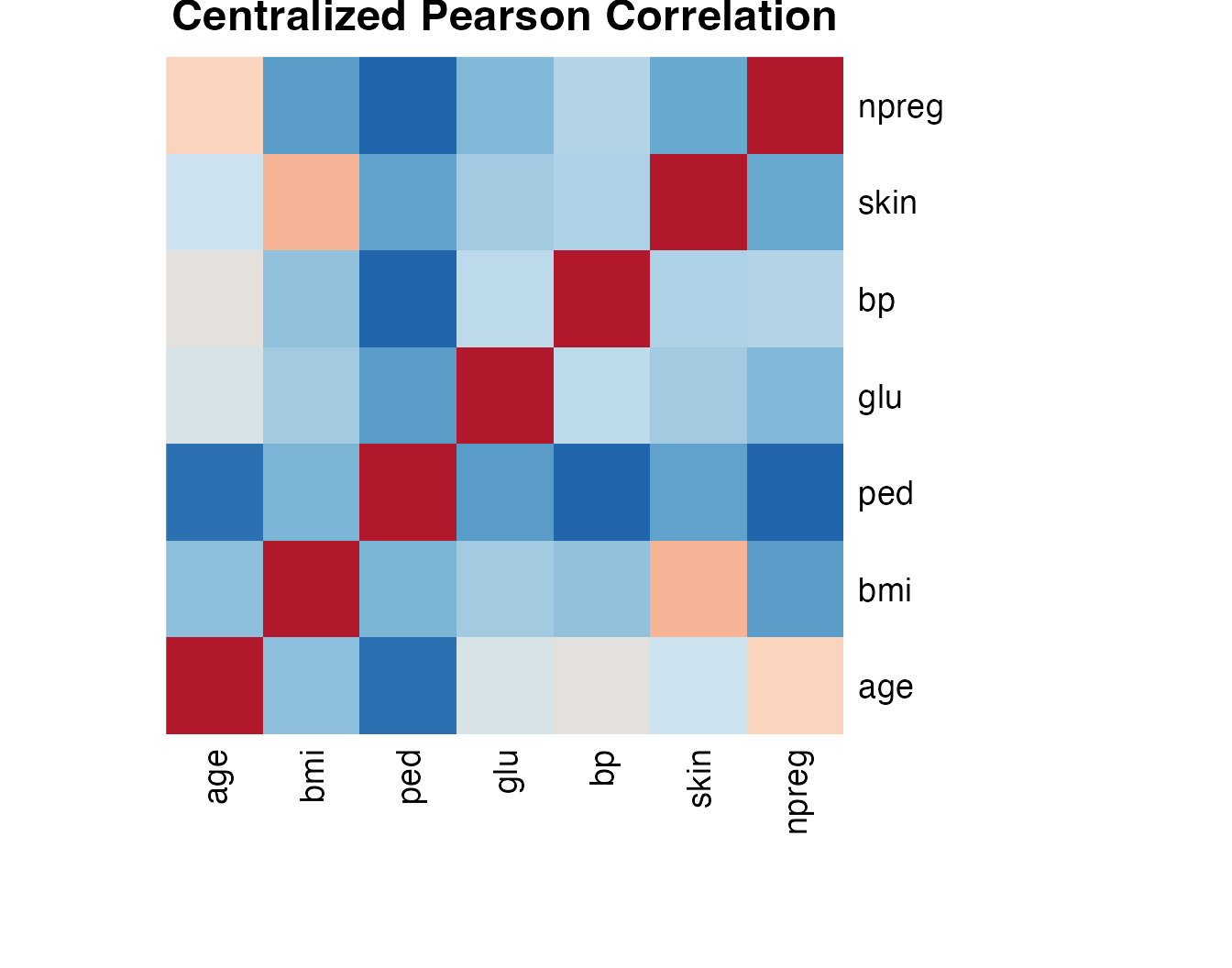

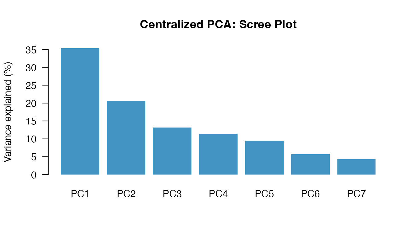
PCA (spectral decomposition)

local_pca <- eigen(local_cor)
local_eigenvalues <- local_pca$values
local_loadings    <- local_pca$vectors
rownames(local_loadings) <- num_vars
colnames(local_loadings) <- paste0("PC", seq_along(num_vars))
local_ve <- local_eigenvalues / sum(local_eigenvalues) * 100

Centralized PCA: eigenvalues and variance explained

Component	Eigenvalue	Variance	Cumulative
PC1	2.4720	35.3%	35.3%
PC2	1.4480	20.7%	56%
PC3	0.9211	13.2%	69.2%
PC4	0.8025	11.5%	80.6%
PC5	0.6568	9.4%	90%
PC6	0.3992	5.7%	95.7%
PC7	0.3004	4.3%	100%

GLM — Gaussian (y = glu)

local_gauss <- glm(glu ~ age + bmi + ped + bp + skin + npreg + diabetes,
                   data = full, family = gaussian)

#> 
#> Call:
#> glm(formula = glu ~ age + bmi + ped + bp + skin + npreg + diabetes, 
#>     family = gaussian, data = full)
#> 
#> Coefficients:
#>              Estimate Std. Error t value Pr(>|t|)    
#> (Intercept) 59.224214  17.124813   3.458 0.000707 ***
#> age          0.601834   0.277074   2.172 0.031419 *  
#> bmi          0.342807   0.460681   0.744 0.457961    
#> ped          1.774110   7.271280   0.244 0.807573    
#> bp           0.403735   0.204122   1.978 0.049771 *  
#> skin        -0.004942   0.245287  -0.020 0.983953    
#> npreg       -0.951066   0.803931  -1.183 0.238673    
#> diabetes    23.457027   5.465637   4.292 3.17e-05 ***
#> ---
#> Signif. codes:  0 '***' 0.001 '**' 0.01 '*' 0.05 '.' 0.1 ' ' 1
#> 
#> (Dispersion parameter for gaussian family taken to be 718.794)
#> 
#>     Null deviance: 148781  on 157  degrees of freedom
#> Residual deviance: 107819  on 150  degrees of freedom
#> AIC: 1497.4
#> 
#> Number of Fisher Scoring iterations: 2

GLM — Binomial (y = diabetes)

local_binom <- glm(diabetes ~ age + bmi + ped + glu + bp + skin + npreg,
                   data = full, family = binomial)

#> 
#> Call:
#> glm(formula = diabetes ~ age + bmi + ped + glu + bp + skin + 
#>     npreg, family = binomial, data = full)
#> 
#> Coefficients:
#>              Estimate Std. Error z value Pr(>|z|)    
#> (Intercept) -9.474861   2.069566  -4.578 4.69e-06 ***
#> age          0.049426   0.025953   1.904 0.056847 .  
#> bmi          0.087041   0.049277   1.766 0.077335 .  
#> ped          1.606924   0.798573   2.012 0.044194 *  
#> glu          0.029988   0.008096   3.704 0.000212 ***
#> bp          -0.018396   0.020518  -0.897 0.369942    
#> skin         0.009106   0.026240   0.347 0.728587    
#> npreg        0.131035   0.073656   1.779 0.075237 .  
#> ---
#> Signif. codes:  0 '***' 0.001 '**' 0.01 '*' 0.05 '.' 0.1 ' ' 1
#> 
#> (Dispersion parameter for binomial family taken to be 1)
#> 
#>     Null deviance: 188.79  on 157  degrees of freedom
#> Residual deviance: 130.11  on 150  degrees of freedom
#> AIC: 146.11
#> 
#> Number of Fisher Scoring iterations: 5

GLM — Poisson (y = npreg)

local_pois <- glm(npreg ~ age + bmi + ped + glu + bp + skin + diabetes,
                  data = full, family = poisson)

#> 
#> Call:
#> glm(formula = npreg ~ age + bmi + ped + glu + bp + skin + diabetes, 
#>     family = poisson, data = full)
#> 
#> Coefficients:
#>               Estimate Std. Error z value Pr(>|z|)    
#> (Intercept)  0.0571560  0.3811101   0.150   0.8808    
#> age          0.0387675  0.0042274   9.171   <2e-16 ***
#> bmi         -0.0008473  0.0096665  -0.088   0.9302    
#> ped         -0.3576770  0.1732612  -2.064   0.0390 *  
#> glu         -0.0030037  0.0016091  -1.867   0.0619 .  
#> bp           0.0053715  0.0042199   1.273   0.2031    
#> skin        -0.0044764  0.0042805  -1.046   0.2957    
#> diabetes     0.3402630  0.1065085   3.195   0.0014 ** 
#> ---
#> Signif. codes:  0 '***' 0.001 '**' 0.01 '*' 0.05 '.' 0.1 ' ' 1
#> 
#> (Dispersion parameter for poisson family taken to be 1)
#> 
#>     Null deviance: 487.64  on 157  degrees of freedom
#> Residual deviance: 327.69  on 150  degrees of freedom
#> AIC: 741.8
#> 
#> Number of Fisher Scoring iterations: 5

---

Federated vertical analysis (dsVert)

We now repeat every analysis using the dsVert federated protocol. Each server only has access to its own subset of variables. Cross-server quantities (such as correlation matrix off-diagonal blocks, and gradients involving variables from multiple servers) are computed under multiparty homomorphic encryption (MHE-CKKS) with threshold decryption, so individual-level data never leaves any server.

Correlation (MHE-CKKS)

The ds.vertCor function computes the full $7 \times 7$ Pearson correlation matrix. Within-server blocks are computed locally; cross-server blocks use CKKS encrypted dot products with threshold decryption and server-side fusion.

variables <- list(
  server1 = c("age", "bmi", "ped"),
  server2 = c("glu", "bp", "skin"),
  server3 = c("npreg")
)

cor_result <- ds.vertCor(
  data_name   = "D_aligned",
  variables   = variables,
  log_n       = 12,
  log_scale   = 40,
  datasources = conns
)

dsvert_cor <- cor_result$correlation

#>           age    bmi     ped    glu      bp   skin   npreg
#> age    1.0000 0.1888 -0.0785 0.3660  0.4253 0.3206  0.5738
#> bmi    0.1888 1.0000  0.1530 0.2371  0.1977 0.6567  0.0625
#> ped   -0.0785 0.1530  1.0000 0.0680 -0.1128 0.0817 -0.1214
#> glu    0.3660 0.2371  0.0680 1.0000  0.2831 0.2365  0.1637
#> bp     0.4253 0.1977 -0.1128 0.2831  1.0000 0.2566  0.2622
#> skin   0.3206 0.6567  0.0817 0.2365  0.2566 1.0000  0.1086
#> npreg  0.5738 0.0625 -0.1214 0.1637  0.2622 0.1086  1.0000

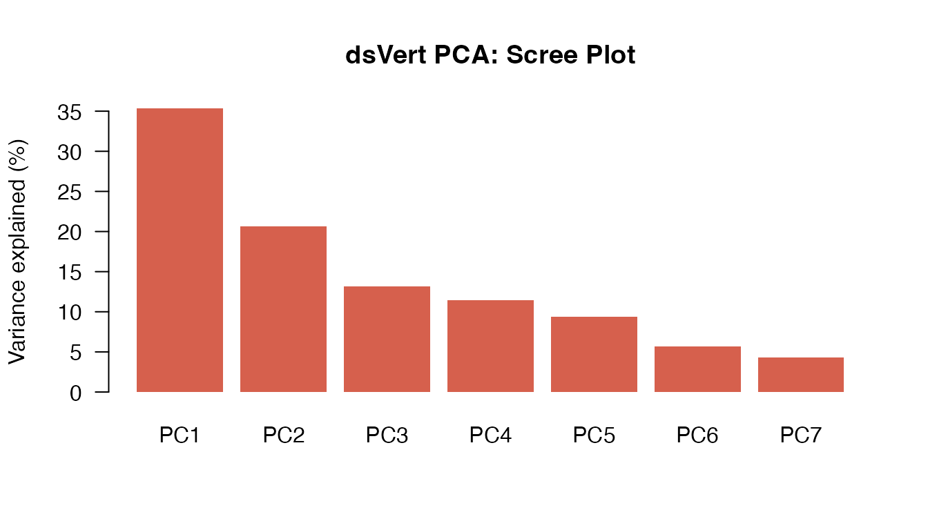
PCA

PCA is computed by eigendecomposition of the federated correlation matrix.

dsvert_pca <- eigen(dsvert_cor)
dsvert_eigenvalues <- dsvert_pca$values
dsvert_loadings    <- dsvert_pca$vectors
rownames(dsvert_loadings) <- num_vars
colnames(dsvert_loadings) <- paste0("PC", seq_along(num_vars))
dsvert_ve <- dsvert_eigenvalues / sum(dsvert_eigenvalues) * 100

dsVert PCA: eigenvalues and variance explained

Component	Eigenvalue	Variance	Cumulative
PC1	2.4720	35.3%	35.3%
PC2	1.4480	20.7%	56%
PC3	0.9211	13.2%	69.2%
PC4	0.8025	11.5%	80.6%
PC5	0.6568	9.4%	90%
PC6	0.3992	5.7%	95.7%
PC7	0.3004	4.3%	100%

GLM — Gaussian (y = glu)

The dsVert GLM uses encrypted-label block coordinate descent (BCD-IRLS). The label variable (glu) resides on server2; the remaining predictors are distributed across all three servers. Gradients are computed under MHE-CKKS and decrypted via share-wrapped threshold decryption with server-side fusion.

glm_gauss <- ds.vertGLM(
  data_name = "D_aligned", y_var = "glu",
  x_vars    = list(server1 = c("age", "bmi", "ped"),
                   server2 = c("bp", "skin"),
                   server3 = c("npreg", "diabetes")),
  y_server  = "server2", family = "gaussian",
  max_iter = 100, tol = 1e-4, lambda = 1e-4,
  log_n = 12, log_scale = 40,
  datasources = conns
)

#> 
#> Vertically Partitioned GLM - Summary
#> ====================================
#> 
#> Call:
#> ds.vertGLM(data_name = "D_aligned", y_var = "glu", x_vars = list(server1 = c("age", 
#>     "bmi", "ped"), server2 = c("bp", "skin"), server3 = c("npreg", 
#>     "diabetes")), y_server = "server2", family = "gaussian", 
#>     max_iter = 100, tol = 1e-04, lambda = 1e-04, log_n = 12, 
#>     log_scale = 40, datasources = conns)
#> 
#> Family: gaussian 
#> Observations: 158 
#> Predictors: 8 
#> Regularization (lambda): 1e-04 
#> Label server: server2 
#> 
#> Convergence:
#>   Iterations: 16 
#>   Converged: TRUE 
#> 
#> Deviance:
#>   Null deviance:     148780.9430  on 157 degrees of freedom
#>   Residual deviance: 107819.5191  on 150 degrees of freedom
#> 
#> Model Fit:
#>   Pseudo R-squared (McFadden): 0.2753 
#>   AIC: 107835.5191 
#> 
#> Coefficients:
#>              Estimate
#> (Intercept) 59.232011
#> age          0.601460
#> bmi          0.342493
#> ped          1.774155
#> bp           0.403806
#> skin        -0.004745
#> npreg       -0.950345
#> diabetes    23.460446

GLM — Binomial (y = diabetes)

Logistic regression with the binary outcome on server3. The IRLS working weights are computed on the label server and routed to non-label servers via transport encryption.

glm_binom <- ds.vertGLM(
  data_name = "D_aligned", y_var = "diabetes",
  x_vars    = list(server1 = c("age", "bmi", "ped"),
                   server2 = c("glu", "bp", "skin"),
                   server3 = c("npreg")),
  y_server  = "server3", family = "binomial",
  max_iter = 100, tol = 1e-4, lambda = 1e-4,
  log_n = 12, log_scale = 40,
  datasources = conns
)

#> 
#> Vertically Partitioned GLM - Summary
#> ====================================
#> 
#> Call:
#> ds.vertGLM(data_name = "D_aligned", y_var = "diabetes", x_vars = list(server1 = c("age", 
#>     "bmi", "ped"), server2 = c("glu", "bp", "skin"), server3 = c("npreg")), 
#>     y_server = "server3", family = "binomial", max_iter = 100, 
#>     tol = 1e-04, lambda = 1e-04, log_n = 12, log_scale = 40, 
#>     datasources = conns)
#> 
#> Family: binomial 
#> Observations: 158 
#> Predictors: 8 
#> Regularization (lambda): 1e-04 
#> Label server: server3 
#> 
#> Convergence:
#>   Iterations: 20 
#>   Converged: TRUE 
#> 
#> Deviance:
#>   Null deviance:     188.7908  on 157 degrees of freedom
#>   Residual deviance: 247.5809  on 150 degrees of freedom
#> 
#> Model Fit:
#>   Pseudo R-squared (McFadden): -0.3114 
#>   AIC: 263.5809 
#> 
#> Coefficients:
#>              Estimate
#> (Intercept) -9.474427
#> age          0.049420
#> bmi          0.087021
#> ped          1.606834
#> glu          0.029989
#> bp          -0.018395
#> skin         0.009116
#> npreg        0.131038

GLM — Poisson (y = npreg)

Count regression for the number of pregnancies. The Poisson log-link compresses the coefficient scale, which tends to aid convergence of the encrypted BCD procedure.

glm_pois <- ds.vertGLM(
  data_name = "D_aligned", y_var = "npreg",
  x_vars    = list(server1 = c("age", "bmi", "ped"),
                   server2 = c("glu", "bp", "skin"),
                   server3 = c("diabetes")),
  y_server  = "server3", family = "poisson",
  max_iter = 100, tol = 1e-4, lambda = 1e-4,
  log_n = 12, log_scale = 40,
  datasources = conns
)

#> 
#> Vertically Partitioned GLM - Summary
#> ====================================
#> 
#> Call:
#> ds.vertGLM(data_name = "D_aligned", y_var = "npreg", x_vars = list(server1 = c("age", 
#>     "bmi", "ped"), server2 = c("glu", "bp", "skin"), server3 = c("diabetes")), 
#>     y_server = "server3", family = "poisson", max_iter = 100, 
#>     tol = 1e-04, lambda = 1e-04, log_n = 12, log_scale = 40, 
#>     datasources = conns)
#> 
#> Family: poisson 
#> Observations: 158 
#> Predictors: 8 
#> Regularization (lambda): 1e-04 
#> Label server: server3 
#> 
#> Convergence:
#>   Iterations: 24 
#>   Converged: TRUE 
#> 
#> Deviance:
#>   Null deviance:     487.6448  on 157 degrees of freedom
#>   Residual deviance: 1354.5837  on 150 degrees of freedom
#> 
#> Model Fit:
#>   Pseudo R-squared (McFadden): -1.7778 
#>   AIC: 1370.5837 
#> 
#> Coefficients:
#>              Estimate
#> (Intercept)  0.057340
#> age          0.038760
#> bmi         -0.000865
#> ped         -0.357688
#> glu         -0.003003
#> bp           0.005376
#> skin        -0.004470
#> diabetes     0.340319

---

Comparative assessment

We now compare the centralized and federated results quantitatively.

Correlation: element-wise differences

cor_diff <- dsvert_cor - local_cor

#>           age      bmi      ped      glu       bp     skin    npreg
#> age   0.0e+00  0.0e+00  0.0e+00  3.5e-06  8.0e-07  4.0e-06  2.9e-06
#> bmi   0.0e+00  0.0e+00  0.0e+00  4.0e-06 -1.6e-06 -8.2e-06  1.8e-06
#> ped   0.0e+00  0.0e+00  0.0e+00 -7.0e-07 -2.4e-06 -9.0e-07 -2.0e-06
#> glu   3.5e-06  4.0e-06 -7.0e-07  0.0e+00  0.0e+00  0.0e+00  3.1e-06
#> bp    8.0e-07 -1.6e-06 -2.4e-06  0.0e+00  0.0e+00  0.0e+00 -1.2e-06
#> skin  4.0e-06 -8.2e-06 -9.0e-07  0.0e+00  0.0e+00  0.0e+00  4.0e-06
#> npreg 2.9e-06  1.8e-06 -2.0e-06  3.1e-06 -1.2e-06  4.0e-06  0.0e+00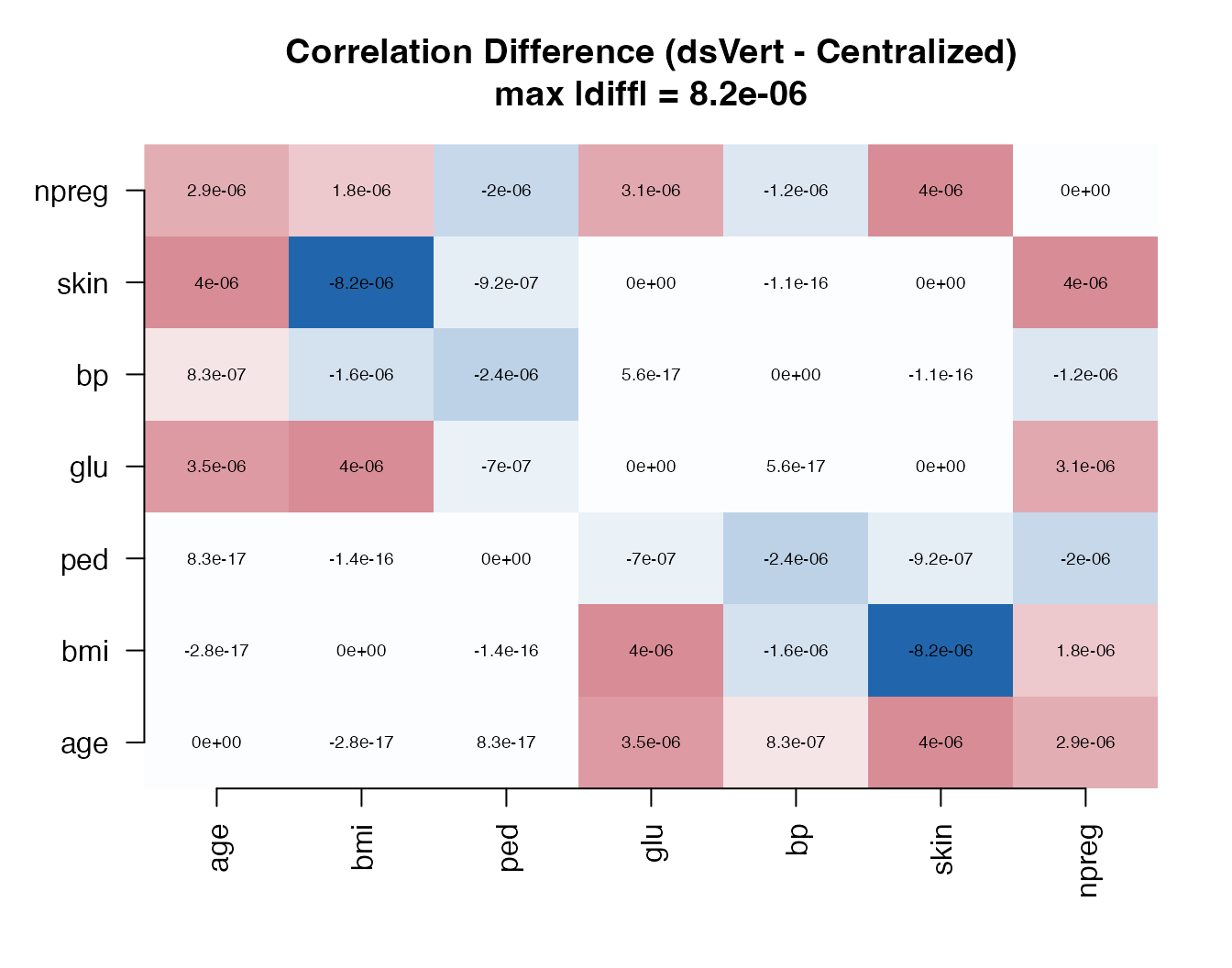

All element-wise differences are of order $10^{-6}$, well below any substantively meaningful threshold.

PCA: eigenvalue comparison

eig_diff <- dsvert_eigenvalues - local_eigenvalues

Eigenvalue comparison (centralized vs. dsVert)

Component	Local	dsVert	Difference
PC1	2.472022	2.472026	4.45e-06
PC2	1.448002	1.447997	-4.97e-06
PC3	0.921104	0.921101	-2.45e-06
PC4	0.802466	0.802465	-1.59e-06
PC5	0.656830	0.656830	4.46e-07
PC6	0.399221	0.399223	2.02e-06
PC7	0.300356	0.300358	2.10e-06

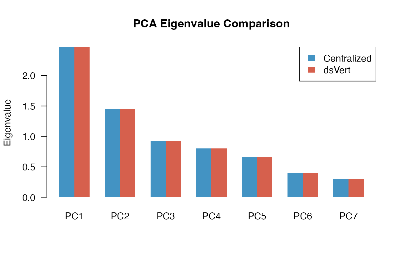
The eigenvalues are virtually identical; differences are of order $10^{-5}$, propagated directly from the correlation matrix precision.

GLM: Gaussian coefficient comparison (y = glu)

gauss_local  <- coef(local_gauss)
gauss_dsvert <- coef(glm_gauss)
gauss_diff   <- gauss_dsvert - gauss_local

Gaussian GLM coefficient comparison (y = glu)

Term	Local	dsVert	Difference
(Intercept)	59.2242	59.2320	7.80e-03
age	0.6018	0.6015	-3.73e-04
bmi	0.3428	0.3425	-3.14e-04
ped	1.7741	1.7742	4.48e-05
bp	0.4037	0.4038	7.08e-05
skin	-0.0049	-0.0047	1.97e-04
npreg	-0.9511	-0.9503	7.20e-04
diabetes	23.4570	23.4604	3.42e-03

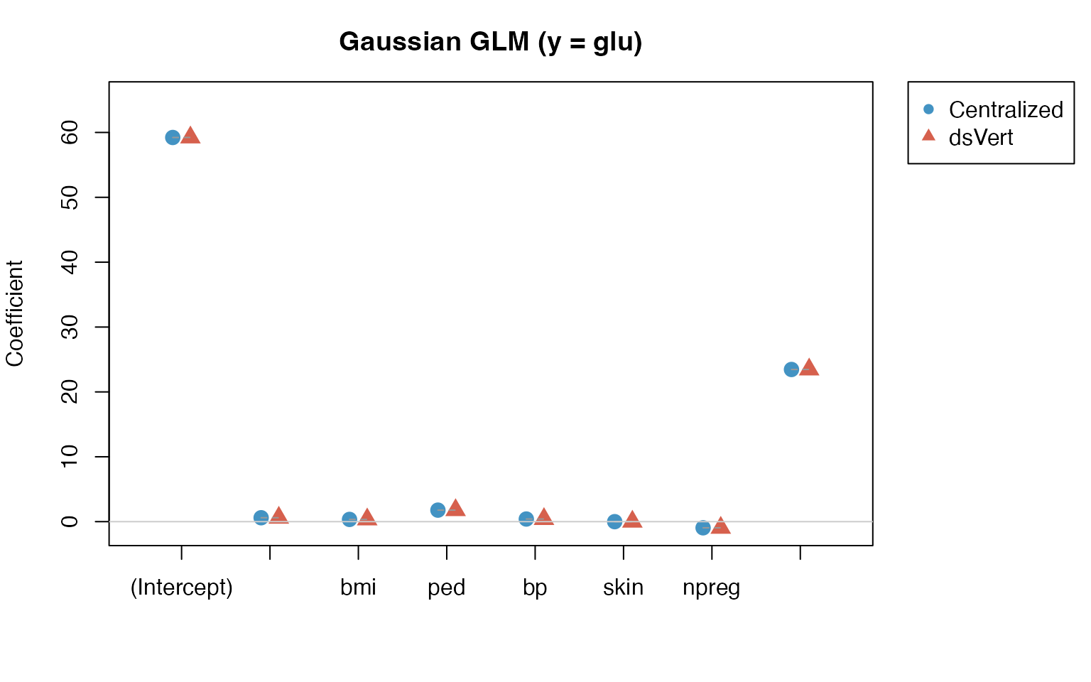
Maximum absolute coefficient difference: 7.8e-03.

GLM: Binomial coefficient comparison (y = diabetes)

binom_local  <- coef(local_binom)
binom_dsvert <- coef(glm_binom)
binom_diff   <- binom_dsvert - binom_local

Binomial GLM coefficient comparison (y = diabetes)

Term	Local	dsVert	Difference
(Intercept)	-9.4749	-9.4744	4.34e-04
age	0.0494	0.0494	-6.52e-06
bmi	0.0870	0.0870	-1.96e-05
ped	1.6069	1.6068	-9.07e-05
glu	0.0300	0.0300	7.05e-07
bp	-0.0184	-0.0184	9.71e-07
skin	0.0091	0.0091	1.09e-05
npreg	0.1310	0.1310	2.81e-06

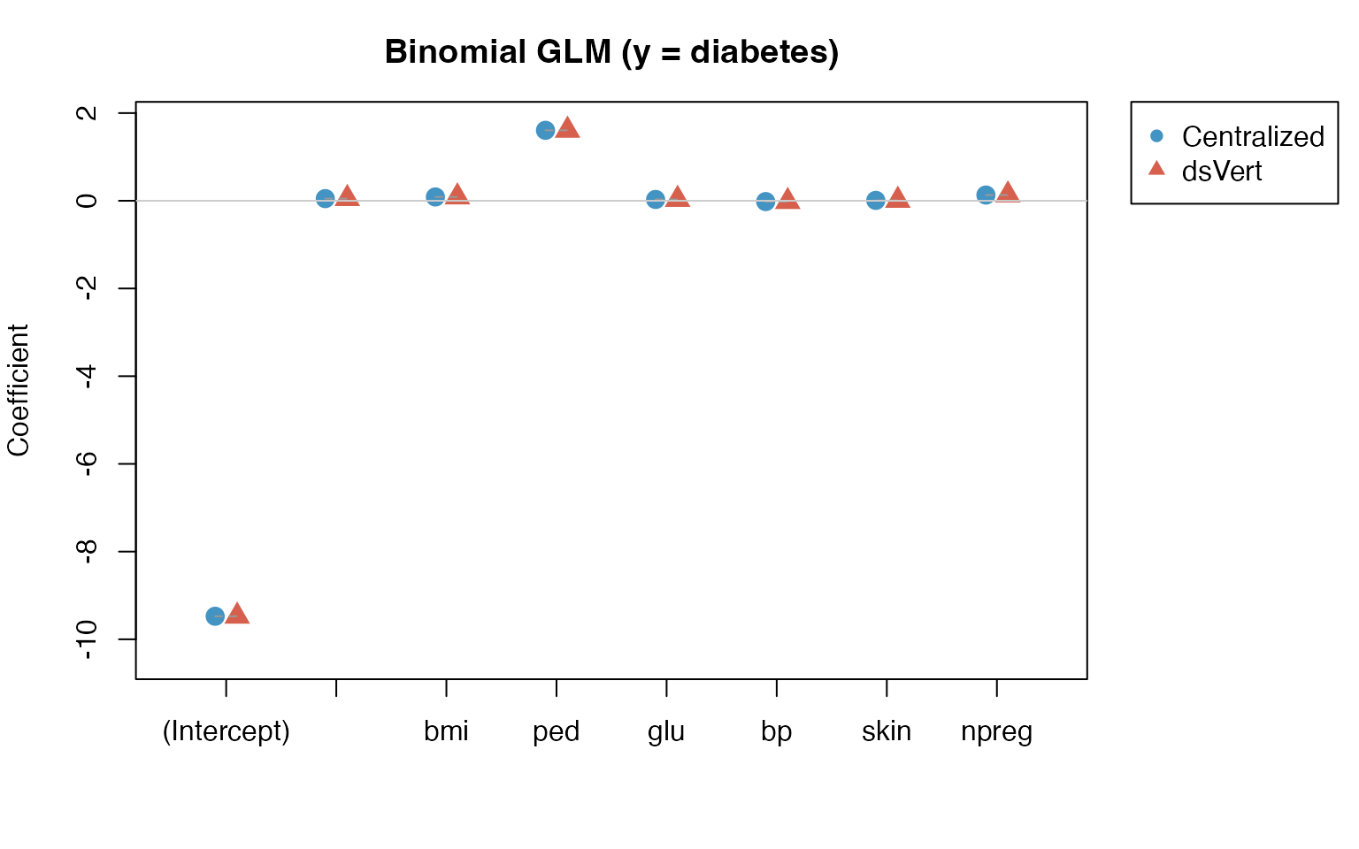
Maximum absolute coefficient difference: 4.34e-04.

GLM: Poisson coefficient comparison (y = npreg)

pois_local  <- coef(local_pois)
pois_dsvert <- coef(glm_pois)
pois_diff   <- pois_dsvert - pois_local

Poisson GLM coefficient comparison (y = npreg)

Term	Local	dsVert	Difference
(Intercept)	0.0572	0.0573	1.84e-04
age	0.0388	0.0388	-7.16e-06
bmi	-0.0008	-0.0009	-1.77e-05
ped	-0.3577	-0.3577	-1.06e-05
glu	-0.0030	-0.0030	1.06e-06
bp	0.0054	0.0054	4.35e-06
skin	-0.0045	-0.0045	6.61e-06
diabetes	0.3403	0.3403	5.64e-05

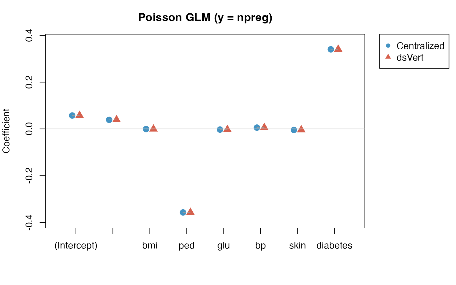
Maximum absolute coefficient difference: 1.84e-04.

Summary

Validation summary (dsVert vs. centralized R)

Protocol	Metric	Value
PSI Alignment	Matched cohort	158 / 200
Correlation	Max |r| error	8.2e-06
PCA	Max eigenvalue error	4.97e-06
GLM Gaussian	Max |coef| error	7.8e-03
GLM Binomial	Max |coef| error	4.34e-04
GLM Poisson	Max |coef| error	1.84e-04

Error analysis

The three error regimes observed correspond to different sources of approximation in the dsVert pipeline:

Correlation and PCA ($\sim 10^{-6}$). These errors arise from CKKS approximate arithmetic used in the MHE threshold protocol. The encoding precision is governed by log_scale = 40, providing approximately $2^{40} \approx 10^{12}$ precision units. After encoding, homomorphic multiplication, inner-sum rotations, and threshold decryption, the effective precision degrades to $\sim 10^{-6}$, consistent with CKKS error propagation theory.

GLM coefficients ($10^{-4}$ to $10^{-3}$). GLM errors are slightly larger because they accumulate over multiple BCD-IRLS iterations, each involving an encrypted gradient computation. Additionally, the ridge regularization parameter ($\lambda = 10^{-4}$) introduces a small systematic bias relative to the unpenalized centralized glm(). The binomial and Poisson families show smaller errors than Gaussian because their link functions (logit, log) compress the coefficient scale.

In all cases, the errors are far below any practically meaningful threshold for statistical inference.